机器学习专栏——（五）线性模型之感知器

线性模型——感知器

    感知器是一个是对生物神经元的模拟，实际上是一个最简单的人工神经网络，即一个人工神经元。作为一个分类算法，感知器常用于处理线性可分的二分类问题。与逻辑回归与softmax回归类似，在进行预测前，都要通过线性回归，然后将线性回归的输出作为激活函数的输入，得到预测值。与逻辑回归和softmax不同之处在于，感知器的标签与激活函数。
    对于感知器，样本的标签表示为 y ∈ { − 1 , + 1 } y \in \{-1,+1\} y∈{−1,+1}。感知器的激活函数为符号函数，表示为：
sgn ( x ) = { − 1    if   w T x <    0 + 1    if   w T x ≥    0 \text{sgn}(x) = \{^{+1 \ \ \ \text {if} \ \ w^Tx \ge \ \ 0}_{-1 \ \ \ \text{if} \ \ w^Tx < \ \ 0} sgn(x)={−1   if  wTx<  0+1   if  wTx≥  0​
    在感知器中，通常使用随机梯度下降算法来更新参数。存在数据集$D$线性可分，存在样本${\mathbf{x}}_{M,1}=[x_1,x_2,...,x_M{]}^T$，其中$M$表示特征数量，数据集的标签为$Y=[y_1,y_1,...y_N{]}^T$，N表示样本数量。得到增广特征向量${\mathbf{x}}_{M+1,1}=[x_1,x_2,...,x_M，1{]}^T$，增广权重向量 ${\mathbf{w}}_{M+1,1}=[w_1,w_2,...,w_M{]}^T$，因此可以得到线性回归输出：
$$Y_{1,1}^L={\mathbf{w}}^{\mathbf{T}}\mathbf{x}$$
    通过上述公式的输出，将其作为符号函数的输入，可以得到预测值：
$${\hat{Y}}_{1,}=\text{sgn}(Y_{1,1}^L)$$
    感知器的更新方式不同于逻辑回归和softmax回归，感知器的更新参数只是发生在预测错误时，也就是说，当预测的结果和真实情况一样，便不会更新参数。当预测有错误时，参数更新公式为：
$${\mathbf{w}}_{M+1,1}^{t+1}={\mathbf{w}}_{M+1,1}^t+\alpha y_i{\mathbf{x}}_{M+1,1}$$
    由参数更新公式可以反推损失函数为：
$$\mathcal{L}=\max (0,-y_i{\mathbf{w}}^{\mathbf{T}}\mathbf{x})$$
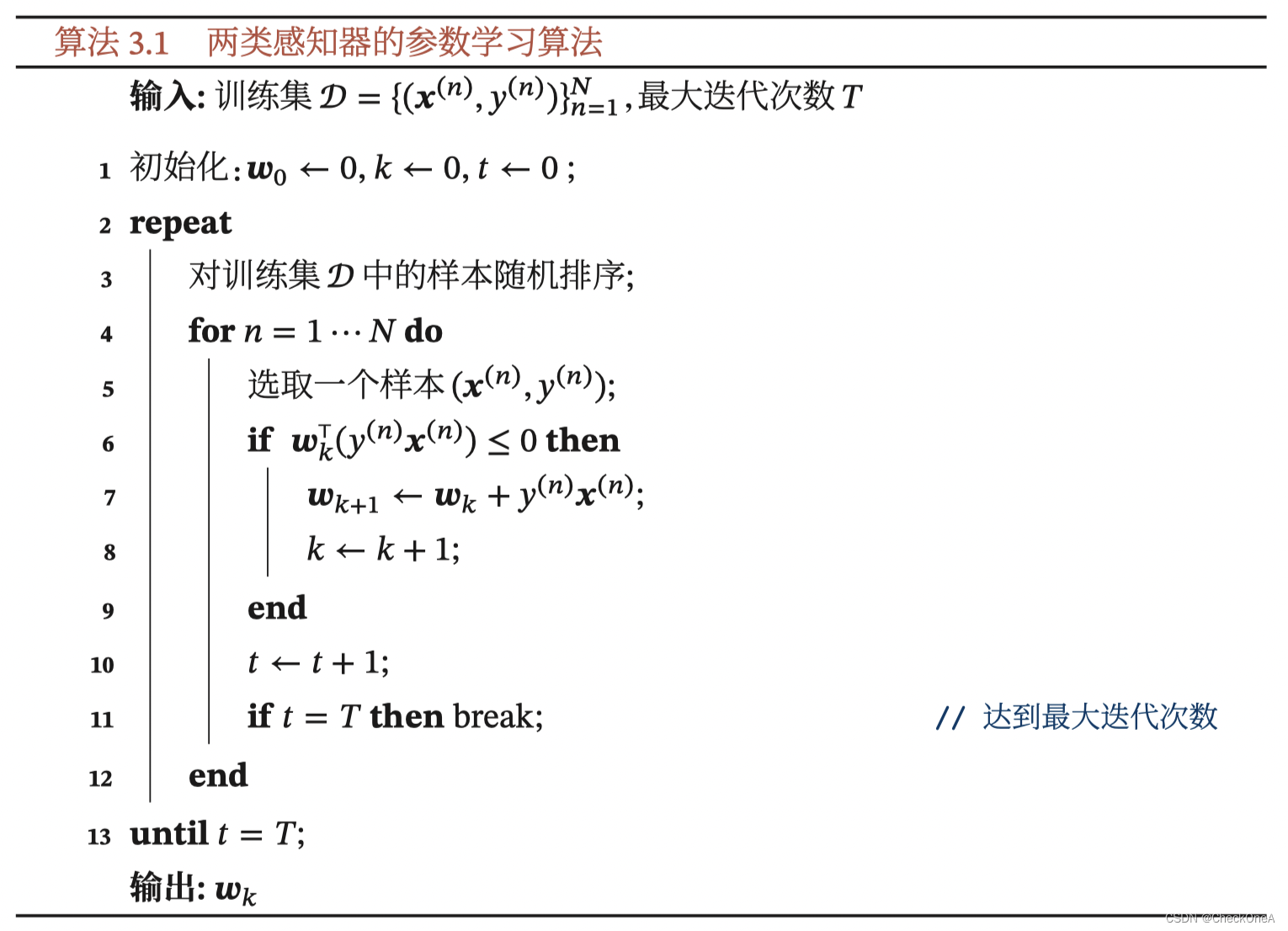
    算法流程[邱锡鹏. 神经网络与深度学习]

    实现代码

"""
@File     :   Perceptron.py   
@Author   :   CheckOneA
@Contact  :   932261247@qq.com
@License  :   (C)Copyright 2018-2021
@Version  :   V1.0
@Date     :   2022/9/12
@Encoding :   UTF-8
@Des      :   None
"""
import numpy as np
from matplotlib import pyplot as plt


class Perceptron:
    def __init__(self, data, interation_max, learning_rate):
        self.data = data
        self.n_data = self.data.shape[0]
        self.n_feature = self.data.shape[1] - 1
        self.interation_max = interation_max
        self.n_data_train = 1
        self.n_feature_train = self.n_feature
        self.lr = learning_rate

    def train(self):
        loss_dis = []
        w = np.random.random(self.n_feature + 1).reshape(-1, 1)
        for interation_index in range(self.interation_max):
            # 获得训练用的数据
            data_train = self.data[np.random.randint(0, self.n_data), :]
            label, feature = self.get_label_feature(data_train)
            line_out = w.T @ feature
            label_pro = self.sgb_function(line_out)
            loss = self.loss_function(-label @ (w.T @ feature))
            loss_dis.append(loss)
            if w.T @ (label * feature) <= 0:
                w = w + self.lr * label * feature
        return w, loss_dis

    def get_label_feature(self, data_train):
        temp = data_train[:][0:2].reshape(-1, 1)
        feature = np.insert(temp, self.n_feature, [1], axis=0)
        label = np.zeros(self.n_data_train)
        for data_index in range(self.n_data_train):
            if data_train[self.n_feature] == 'setosa':
                label[data_index] = 1
            else:
                label[data_index] = -1
        return label, feature

    @staticmethod
    def sgb_function(input_data):
        return np.sign(input_data)

    def loss_function(self, input_data):
        temp = np.zeros_like(input_data)
        loss = np.maximum(temp, input_data)
        return np.sum(loss) / self.n_data_train ** 2

    @ staticmethod
    def plot_loss(loss):
        plt.figure()
        x = np.linspace(1, len(loss), len(loss))
        plt.plot(x, loss, color='r')
        plt.xlabel("interation")
        plt.ylabel("Loss")
        plt.show()

    def plot_data(self, w):
        plt.figure()
        x = np.linspace(4, 7)
        a = -w[0] / w[1]
        b = - w[2] / w[1]
        y = a * x + b
        plt.plot(x, y, color='r')
        x1 = self.data[:, 0]
        x2 = self.data[:, 1]
        for data_index in range(len(x1)):
            flag = a * x1[data_index] + b - x2[data_index]
            if flag > 0:
                plt.scatter(x1[data_index], x2[data_index], color='b')
            elif flag <= 0:
                plt.scatter(x1[data_index], x2[data_index], color='m')
        plt.show()

    测试代码

import matplotlib.pyplot as plt
import numpy as np
import pandas as pd

from Perceptron import Perceptron

if __name__ == '__main__':
    data_df = pd.read_csv("Data/iris.csv",
                          usecols=["Sepal.Length", "Sepal.Width", "Species"])
    data_np = data_df.to_numpy()

    perceptron = Perceptron(data=data_np,
                            interation_max=60000,
                            learning_rate=0.001)
    w, loss = perceptron.train()
    perceptron.plot_loss(loss)
    perceptron.plot_data(w)

    训练结果