


在我们的计算机系统中,每个字符将占用1字节(8位)。给定一个字符串‘ AAABBCCCCCDDDAAAAA’,请使用 Huffman 编码来压缩它。构造哈夫曼树并确定每个符号的代码。对于这个问题,您可以手绘树的建设过程,并采取一张照片,包括在您的文件。

哈弗曼编码前所需要的位数:20byte,也就是102420位;哈弗曼编码后所需要的位数:6byte,也就是61024位
计算图像压缩率代码如下:
import os
import cv2
from queue import PriorityQueue
import numpy as np
import math
import struct
import matplotlib.pyplot as plt
'''
对图像哈夫曼编码/解码
根据哈夫曼编码灰度图像,保存到文件中;读取哈夫曼编码的文件,解码成图像,与原图像对比。
'''
class HuffmanNode(object):
'''
哈夫曼树的节点类
'''
def __init__(self, value, key=None, symbol='', left_child=None, right_child=None):
'''
初始化哈夫曼树的节点
:param value: 节点的值,i.e. 元素出现的频率
:param key: 节点代表的元素,非叶子节点为None
:param symbol: 节点的哈夫曼编码,初始化必须为空字符串
:param left_child: 左子节点
:param right_child: 右子节点
'''
self.left_child = left_child
self.right_child = right_child
self.value = value
self.key = key
assert symbol == ''
self.symbol = symbol
def __eq__(self, other):
'''
用于比较两个HuffmanNode的大小,等于号,根据value的值比较
:param other:
:return:
'''
return self.value == other.value
def __gt__(self, other):
'''
用于比较两个HuffmanNode的大小,大于号,根据value的值比较
:param other:
:return:
'''
return self.value > other.value
def __lt__(self, other):
'''
用于比较两个HuffmanNode的大小,小于号,根据value的值比较
:param other:
:return:
'''
return self.value < other.value
def createTree(hist_dict: dict) -> HuffmanNode:
'''
构造哈夫曼树
可以写一个HuffmanTree的类
:param hist_dict: 图像的直方图,dict = {pixel_value: count}
:return: HuffmanNode, 哈夫曼树的根节点
'''
# 借助优先级队列实现直方图频率的排序,取出和插入元素很方便
q = PriorityQueue()
# 根据传入的像素值和频率字典构造哈夫曼节点并放入队列中
for k, v in hist_dict.items():
# 这里放入的都是之后哈夫曼树的叶子节点,key都是各自的元素
q.put(HuffmanNode(value=v, key=k))
# 判断条件,直到队列中只剩下一个根节点
while q.qsize() > 1:
# 取出两个最小的哈夫曼节点,队列中这两个节点就不在了
l_freq, r_freq = q.get(), q.get()
# 增加他们的父节点,父节点值为这两个哈夫曼节点的和,但是没有key值;左子节点是较小的,右子节点是较大的
node = HuffmanNode(value=l_freq.value + r_freq.value, left_child=l_freq, right_child=r_freq)
# 把构造的父节点放在队列中,继续排序和取放、构造其他的节点
q.put(node)
# 队列中只剩下根节点了,返回根节点
return q.get()
def walkTree_VLR(root_node: HuffmanNode, symbol=''):
'''
前序遍历一个哈夫曼树,同时得到每个元素(叶子节点)的编码,保存到全局的Huffman_encode_dict
:param root_node: 哈夫曼树的根节点
:param symbol: 用于对哈夫曼树上的节点进行编码,递归的时候用到,为'0'或'1'
:return: None
'''
# 为了不增加变量复制的成本,直接使用一个dict类型的全局变量保存每个元素对应的哈夫曼编码
global Huffman_encode_dict
# 判断节点是不是HuffmanNode,因为叶子节点的子节点是None
if isinstance(root_node, HuffmanNode):
# 编码操作,改变每个子树的根节点的哈夫曼编码,根据遍历过程是逐渐增加编码长度到完整的
root_node.symbol += symbol
# 判断是否走到了叶子节点,叶子节点的key!=None
if root_node.key != None:
# 记录叶子节点的编码到全局的dict中
Huffman_encode_dict[root_node.key] = root_node.symbol
# 访问左子树,左子树在此根节点基础上赋值'0'
walkTree_VLR(root_node.left_child, symbol=root_node.symbol + '0')
# 访问右子树,右子树在此根节点基础上赋值'1'
walkTree_VLR(root_node.right_child, symbol=root_node.symbol + '1')
return
def encodeImage(src_img: np.ndarray, encode_dict: dict):
'''
用已知的编码字典对图像进行编码
:param src_img: 原始图像数据,必须是一个向量
:param encode_dict: 编码字典,dict={element:code}
:return: 图像编码后的字符串,字符串中只包含'0'和'1'
'''
img_encode = ""
assert len(src_img.shape) == 1, '`src_img` must be a vector'
for pixel in src_img:
img_encode += encode_dict[pixel]
return img_encode
def writeBinImage(img_encode: str, huffman_file: str):
'''
把编码后的二进制图像数据写入到文件中
:param img_encode: 图像编码字符串,只包含'0'和'1'
:param huffman_file: 要写入的图像编码数据文件的路径
:return:
'''
# 文件要以二进制打开
with open(huffman_file, 'wb') as f:
# 每8个bit组成一个byte
for i in range(0, len(img_encode), 8):
# 把这一个字节的数据根据二进制翻译为十进制的数字
img_encode_dec = int(img_encode[i:i + 8], 2)
# 把这一个字节的十进制数据打包为一个unsigned char,大端(可省略)
img_encode_bin = struct.pack('>B', img_encode_dec)
# 写入这一个字节数据
f.write(img_encode_bin)
def readBinImage(huffman_file: str, img_encode_len: int):
'''
从二进制的编码文件读取数据,得到原来的编码信息,为只包含'0'和'1'的字符串
:param huffman_file: 保存的编码文件
:param img_encode_len: 原始编码的长度,必须要给出,否则最后一个字节对不上
:return: str,只包含'0'和'1'的编码字符串
'''
code_bin_str = ""
with open(huffman_file, 'rb') as f:
# 从文件读取二进制数据
content = f.read()
# 从二进制数据解包到十进制数据,所有数据组成的是tuple
code_dec_tuple = struct.unpack('>' + 'B' * len(content), content)
for code_dec in code_dec_tuple:
# 通过bin把解压的十进制数据翻译为二进制的字符串,并填充为8位,否则会丢失高位的0
# 0 -> bin() -> '0b0' -> [2:] -> '0' -> zfill(8) -> '00000000'
code_bin_str += bin(code_dec)[2:].zfill(8)
# 由于原始的编码最后可能不足8位,保存到一个字节的时候会在高位自动填充0,读取的时候需要去掉填充的0,否则读取出的编码会比原来的编码长
# 计算读取的编码字符串与原始编码字符串长度的差,差出现在读取的编码字符串的最后一个字节,去掉高位的相应数量的0就可以
len_diff = len(code_bin_str) - img_encode_len
# 在读取的编码字符串最后8位去掉高位的多余的0
code_bin_str = code_bin_str[:-8] + code_bin_str[-(8 - len_diff):]
return code_bin_str
def decodeHuffman(img_encode: str, huffman_tree_root: HuffmanNode):
'''
根据哈夫曼树对编码数据进行解码
:param img_encode: 哈夫曼编码数据,只包含'0'和'1'的字符串
:param huffman_tree_root: 对应的哈夫曼树,根节点
:return: 原始图像数据展开的向量
'''
img_src_val_list = []
# 从根节点开始访问
root_node = huffman_tree_root
# 每次访问都要使用一位编码
for code in img_encode:
# 如果编码是'0',说明应该走到左子树
if code == '0':
root_node = root_node.left_child
# 如果编码是'1',说明应该走到右子树
elif code == '1':
root_node = root_node.right_child
# 只有叶子节点的key才不是None,判断当前走到的节点是不是叶子节点
if root_node.key != None:
# 如果是叶子节点,则记录这个节点的key,也就是哪个原始数据的元素
img_src_val_list.append(root_node.key)
# 访问到叶子节点之后,下一次应该从整个数的根节点开始访问了
root_node = huffman_tree_root
return np.asarray(img_src_val_list)
def decodeHuffmanByDict(img_encode: str, encode_dict: dict):
'''
另外一种解码策略是先遍历一遍哈夫曼树得到所有叶子节点编码对应的元素,可以保存在字典中,再对字符串的子串逐个与字典的键进行比对,就得到相应的元素是什么。
用C语言也可以这么做。
这里不再对哈夫曼树重新遍历了,因为之前已经遍历过,所以直接使用之前记录的编码字典就可以。
:param img_encode: 哈夫曼编码数据,只包含'0'和'1'的字符串
:param encode_dict: 编码字典dict={element:code}
:return: 原始图像数据展开的向量
'''
img_src_val_list = []
decode_dict = {}
# 构造一个key-value互换的字典,i.e. dict={code:element},后边方便使用
for k, v in encode_dict.items():
decode_dict[v] = k
# s用来记录当前字符串的访问位置,相当于一个指针
s = 0
# 只要没有访问到最后
while len(img_encode) > s + 1:
# 遍历字典中每一个键code
for k in decode_dict.keys():
# 如果当前的code字符串与编码字符串前k个字符相同,k表示code字符串的长度,那么就可以确定这k个编码对应的元素是什么
if k == img_encode[s:s + len(k)]:
img_src_val_list.append(decode_dict[k])
# 指针移动k个单位
s += len(k)
# 如果已经找到了相应的编码了,就可以找下一个了
break
return np.asarray(img_src_val_list)
def put(path):
# 即使原图像是灰度图,也需要加入GRAYSCALE标志
src_img = cv2.imread(path, cv2.IMREAD_GRAYSCALE)
# 记录原始图像的尺寸,后续还原图像要用到
src_img_w, src_img_h = src_img.shape[:2]
# 把图像展开成一个行向量
src_img_ravel = src_img.ravel()
# {pixel_value:count},保存原始图像每个像素对应出现的次数,也就是直方图
hist_dict = {}
# 得到原始图像的直方图,出现次数为0的元素(像素值)没有加入
for p in src_img_ravel:
if p not in hist_dict:
hist_dict[p] = 1
else:
hist_dict[p] += 1
# 构造哈夫曼树
huffman_root_node = createTree(hist_dict)
# 遍历哈夫曼树,并得到每个元素的编码,保存到Huffman_encode_dict,这是全局变量
walkTree_VLR(huffman_root_node)
global Huffman_encode_dict
print('哈夫曼编码字典:', Huffman_encode_dict)
# 根据编码字典编码原始图像得到二进制编码数据字符串
img_encode = encodeImage(src_img_ravel, Huffman_encode_dict)
# 把二进制编码数据字符串写入到文件中,后缀为bin
writeBinImage(img_encode, 'huffman_bin_img_file.bin')
# 读取编码的文件,得到二进制编码数据字符串
img_read_code = readBinImage('huffman_bin_img_file.bin', len(img_encode))
# 解码二进制编码数据字符串,得到原始图像展开的向量
# 这是根据哈夫曼树进行解码的方式
img_src_val_array = decodeHuffman(img_read_code, huffman_root_node)
# 这是根据编码字典进行解码的方式,更慢一些
# img_src_val_array = decodeHuffmanByDict(img_read_code, Huffman_encode_dict)
# 确保解码的数据与原始数据大小一致
assert len(img_src_val_array) == src_img_w * src_img_h
# 恢复原始二维图像
img_decode = np.reshape(img_src_val_array, [src_img_w, src_img_h])
# 计算平均编码长度和编码效率
total_code_len = 0
total_code_num = sum(hist_dict.values())
avg_code_len = 0
I_entropy = 0
for key in hist_dict.keys():
count = hist_dict[key]
code_len = len(Huffman_encode_dict[key])
prob = count / total_code_num
avg_code_len += prob * code_len
I_entropy += -(prob * math.log2(prob))
S_eff = I_entropy / avg_code_len
print("平均编码长度为:{:.3f}".format(avg_code_len))
print("编码效率为:{:.6f}".format(S_eff))
# 压缩率
ori_size = src_img_w * src_img_h * 8 / (1024 * 8)
comp_size = len(img_encode) / (1024 * 8)
comp_rate = 1 - comp_size / ori_size
print('原图灰度图大小', ori_size, 'KB 压缩后大小', comp_size, 'KB 压缩率', comp_rate, '%')
plt.rcParams['font.sans-serif'] = ['SimHei']
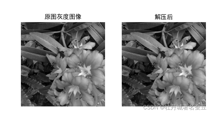
plt.subplot(121), plt.imshow(src_img, plt.cm.gray), plt.title('原图灰度图像'), plt.axis('off')
plt.subplot(122), plt.imshow(img_decode, plt.cm.gray), plt.title('解压后'), plt.axis('off')
# plt.savefig('1.1new.jpg')
plt.show()
if __name__ == '__main__':
# 哈夫曼编码字典{pixel_value:code},在函数中作为全局变量用到了
Huffman_encode_dict = {}
# 图像处理函数,要传入路径
put(r'./1.bmp')
哈夫曼编码字典: {199: ‘0000000000’, 219: ‘0000000001000’, 224: ‘0000000001001’, 211: ‘000000000101’, 223: ‘0000000001100’, 241: ‘000000000110100’, 245: ‘000000000110101’, 236: ‘00000000011011’, 208: ‘000000000111’, 183: ‘000000001’, 180: ‘000000010’, 198: ‘0000000110’, 197: ‘0000000111’, 145: ‘0000001’, 95: ‘0000010’, 167: ‘00000110’, 9: ‘00000111’, 32: ‘0000100’, 168: ‘00001010’, 181: ‘000010110’, 178: ‘000010111’, 148: ‘0000110’, 33: ‘0000111’, 101: ‘0001000’, 100: ‘0001001’, 143: ‘0001010’, 98: ‘0001011’, 99: ‘0001100’, 146: ‘0001101’, 147: ‘0001110’, 166: ‘00011110’, 179: ‘000111110’, 210: ‘000111111000’, 221: ‘0001111110010’, 225: ‘0001111110011’, 203: ‘00011111101’, 196: ‘0001111111’, 104: ‘0010000’, 103: ‘0010001’, 35: ‘0010010’, 102: ‘0010011’, 96: ‘0010100’, 97: ‘0010101’, 56: ‘0010110’, 55: ‘0010111’, 34: ‘0011000’, 36: ‘0011001’, 142: ‘0011010’, 105: ‘0011011’, 144: ‘0011100’, 165: ‘00111010’, 10: ‘00111011’, 54: ‘0011110’, 177: ‘001111100’, 5: ‘001111101’, 11: ‘00111111’, 49: ‘0100000’, 139: ‘0100001’, 137: ‘0100010’, 50: ‘0100011’, 45: ‘0100100’, 39: ‘0100101’, 140: ‘0100110’, 44: ‘0100111’, 46: ‘0101000’, 163: ‘01010010’, 3: ‘010100110’, 176: ‘010100111’, 47: ‘0101010’, 51: ‘0101011’, 141: ‘0101100’, 48: ‘0101101’, 52: ‘0101110’, 106: ‘0101111’, 136: ‘0110000’, 38: ‘0110001’, 43: ‘0110010’, 108: ‘0110011’, 37: ‘0110100’, 53: ‘0110101’, 138: ‘0110110’, 4: ‘011011100’, 206: ‘011011101000’, 218: ‘0110111010010’, 235: ‘01101110100110’, 244: ‘01101110100111’, 222: ‘0110111010100’, 220: ‘0110111010101’, 205: ‘011011101011’, 230: ‘01101110110000’, 238: ‘01101110110001’, 217: ‘0110111011001’, 207: ‘011011101101’, 213: ‘0110111011100’, 228: ‘0110111011101’, 215: ‘0110111011110’, 212: ‘0110111011111’, 12: ‘01101111’, 107: ‘0111000’, 42: ‘0111001’, 40: ‘0111010’, 41: ‘0111011’, 164: ‘01111000’, 13: ‘01111001’, 109: ‘0111101’, 110: ‘0111110’, 135: ‘0111111’, 175: ‘100000000’, 195: ‘1000000010’, 194: ‘1000000011’, 24: ‘10000001’, 133: ‘1000001’, 25: ‘10000100’, 14: ‘10000101’, 111: ‘1000011’, 119: ‘1000100’, 134: ‘1000101’, 132: ‘1000110’, 120: ‘1000111’, 117: ‘1001000’, 113: ‘1001001’, 161: ‘10010100’, 162: ‘10010101’, 115: ‘1001011’, 123: ‘1001100’, 15: ‘10011010’, 16: ‘10011011’, 124: ‘1001110’, 26: ‘10011110’, 160: ‘10011111’, 112: ‘1010000’, 114: ‘1010001’, 121: ‘1010010’, 118: ‘1010011’, 6: ‘101010000’, 2: ‘101010001’, 72: ‘10101001’, 122: ‘1010101’, 116: ‘1010110’, 131: ‘1010111’, 130: ‘1011000’, 193: ‘1011001000’, 191: ‘1011001001’, 174: ‘101100101’, 71: ‘10110011’, 125: ‘1011010’, 240: ‘101101100000000’, 250: ‘1011011000000010’, 246: ‘10110110000000110’, 254: ‘10110110000000111’, 251: ‘101101100000010’, 233: ‘101101100000011’, 243: ‘101101100000100’, 247: ‘101101100000101’, 227: ‘10110110000011’, 204: ‘101101100001’, 202: ‘10110110001’, 190: ‘1011011001’, 173: ‘101101101’, 27: ‘10110111’, 129: ‘1011100’, 74: ‘10111010’, 70: ‘10111011’, 69: ‘10111100’, 20: ‘10111101’, 19: ‘10111110’, 17: ‘10111111’, 128: ‘1100000’, 126: ‘1100001’, 28: ‘11000100’, 172: ‘110001010’, 184: ‘1100010110’, 192: ‘1100010111’, 73: ‘11000110’, 76: ‘11000111’, 127: ‘1100100’, 83: ‘11001010’, 159: ‘11001011’, 67: ‘11001100’, 155: ‘11001101’, 157: ‘11001110’, 86: ‘11001111’, 87: ‘11010000’, 21: ‘11010001’, 75: ‘11010010’, 68: ‘11010011’, 82: ‘11010100’, 64: ‘11010101’, 154: ‘11010110’, 84: ‘11010111’, 80: ‘11011000’, 77: ‘11011001’, 1: ‘110110100’, 7: ‘110110101’, 78: ‘11011011’, 23: ‘11011100’, 29: ‘11011101’, 156: ‘11011110’, 88: ‘11011111’, 65: ‘11100000’, 85: ‘11100001’, 187: ‘1110001000’, 189: ‘1110001001’, 214: ‘11100010100000’, 253: ‘11100010100001’, 209: ‘1110001010001’, 0: ‘111000101001’, 201: ‘11100010101’, 185: ‘1110001011’, 153: ‘11100011’, 18: ‘11100100’, 81: ‘11100101’, 158: ‘11100110’, 63: ‘11100111’, 61: ‘11101000’, 58: ‘11101001’, 79: ‘11101010’, 66: ‘11101011’, 22: ‘11101100’, 62: ‘11101101’, 186: ‘1110111000’, 188: ‘1110111001’, 169: ‘111011101’, 60: ‘11101111’, 59: ‘11110000’, 171: ‘111100010’, 170: ‘111100011’, 89: ‘11110010’, 91: ‘11110011’, 92: ‘11110100’, 152: ‘11110101’, 93: ‘11110110’, 150: ‘11110111’, 90: ‘11111000’, 30: ‘11111001’, 252: ‘111110100000000’, 249: ‘111110100000001’, 242: ‘111110100000010’, 248: ‘1111101000000110’, 237: ‘1111101000000111’, 232: ‘11111010000010’, 231: ‘11111010000011’, 229: ‘11111010000100’, 226: ‘11111010000101’, 234: ‘111110100001100’, 239: ‘111110100001101’, 216: ‘11111010000111’, 200: ‘11111010001’, 182: ‘1111101001’, 8: ‘111110101’, 57: ‘11111011’, 151: ‘11111100’, 94: ‘11111101’, 149: ‘11111110’, 31: ‘11111111’}
平均编码长度为:7.544
编码效率为:0.997191
原图灰度图大小 256.0 KB 压缩后大小 241.4217529296875 KB 压缩率 0.0569462776184082 %
今天的分享到此结束,希望对您有所帮助!!!!!


 9662
9662


 被折叠的 条评论
为什么被折叠?
被折叠的 条评论
为什么被折叠?
 到【灌水乐园】发言


