吴恩达线性回归复习

sigmoid函数

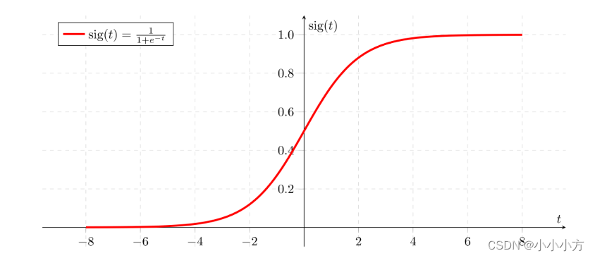
 在深度学习中很少使用数学库，因为函数的输入是实数，深度学习主要使用的是矩阵和向量。

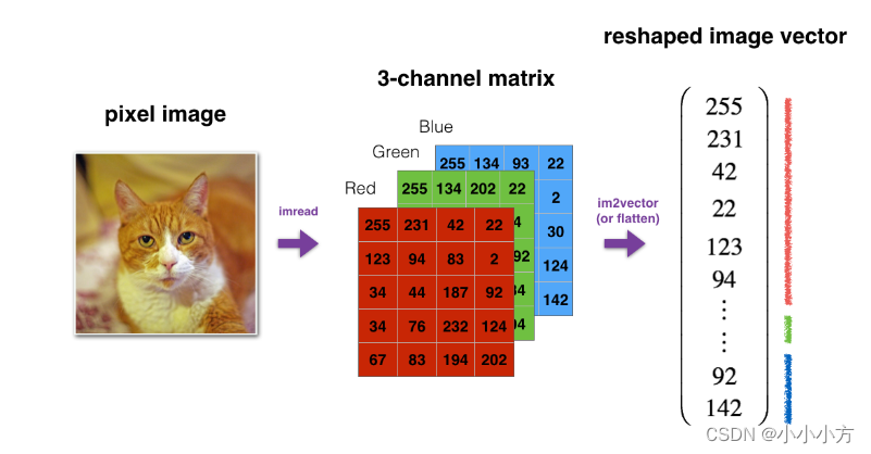
3D图像一般为(length,height,depth)，作为算法输入时，转换为(length*height*depth,1)

 对数据进行标准化之后，可以带来更好的性能，因为梯度下降在归一化后收敛的更快。将x更改为。

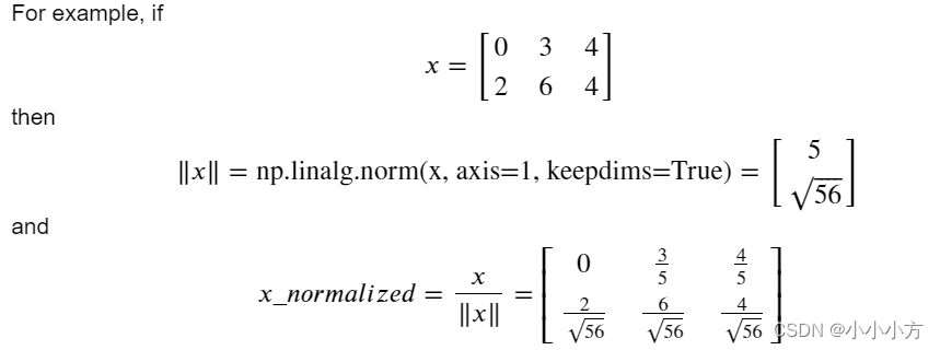
 axis=1代表按照行进行标准化，keepdims=true代表应用广播机制。

softmax函数视为算法需要对两个或更多类进行分类时使用的归一化函数。

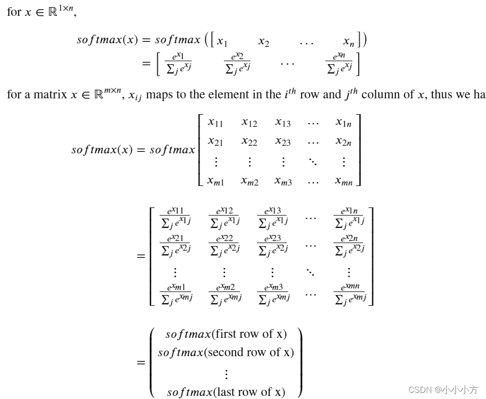
 m代表训练示例的数量，每行都有相同特征的数据。应该对每个训练示例的所有特征进行归一化，因此应该对列执行softmax。

使用矢量化，确保代码的计算效率。

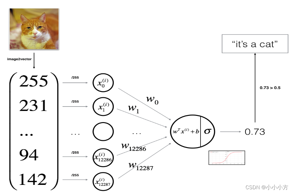
构建一个见到那的图像识别算法，改算法可以正确的将图片分类为猫或者非猫。

import numpy as np
import copy
import matplotlib.pyplot as plt
import h5py
import scipy
from PIL import Image
from scipy import ndimage
from lr_utils import load_dataset
from public_tests import *

%matplotlib inline
%load_ext autoreload
%autoreload 2


m_train = train_set_x_orig.shape[0]
m_test = test_set_x_orig.shape[0]
num_px = train_set_x_orig.shape[1]

# 重塑训练和测试数据集
# 参数-1自行计算剩余维度
train_set_x_flatten = train_set_x_orig.reshape(train_set_x_orig.shape[0],-1).T
test_set_x_flatten = test_set_x_orig.reshape(test_set_x_orig.shape[0],-1).T

# 预处理步骤：集中和标准化数据集，从每个示例中减去整个numpy数组的平均值
# 然后将每个示例除以整个numpy数组的标准差
# 对于图片数据集，将数据集的每一行除以255就更简单
train_set_x = train_set_x_flatten / 255.
test_set_x = test_set_x_flatten / 255.

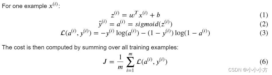
逻辑回归是最简单的神经网络

 

#sigmoid函数
def sigmoid(z):
    s= 1/(1+np.exp(-z))
    return s

# 初始化参数
def initialize_with_zeros(dim):
     w=np.zeros((dim,1))
     b=0.0
    return w,b

# 前向传播和后向传播
def propagate(w,b,X,Y):
    m = X.shape[1]
    A = sigmoid(np.dot(w.T,X)+b)
    cost = -1/m*np.sum(Y*np.log(A)+(1-Y)*np.log(1-A))
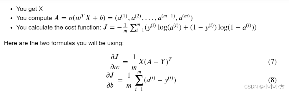
    dw=1/m*np.dot(X,(A-Y).T)
    db=1/m*np.sum(A-Y)
    cost = np.squeeze(np.array(cost))
    grads = {"dw": dw,
             "db": db}
    return grads, cost

# 优化
def optimize(w, b, X, Y, num_iterations=100, learning_rate=0.009, print_cost=False):
    w = copy.deepcopy(w)
    b = copy.deepcopy(b)
    costs = []
    for i in range(num_iterations):
        grads,cost=propagate(w,b,X,Y)
        dw = grads["dw"]
        db = grads["db"]
        w=w-learning_rate*dw
        b=b-learning_rate*db
        if i % 100 == 0:
                costs.append(cost)  
                if print_cost:
                      print ("Cost after iteration %i: %f" %(i, cost))
        params = {"w": w,
              "b": b}
    
        grads = {"dw": dw,
               "db": db}
      
    return params, grads, costs

# 预测
def predict(w,b,X):
    m = X.shape[1]
    Y_prediction = np.zeros((1, m))
    w = w.reshape(X.shape[0], 1)
    A=sigmoid(np.dot(w.T,X)+b)
    for i in range(A.shape[1]):
        if A[0,i] <= 0.5:
            Y_prediction[0,i]=0
        else:
            Y_prediction[0,i]=1
   return Y_prediction  

# 画出曲线
costs = np.squeeze(logistic_regression_model['costs'])
plt.plot(costs)
plt.ylabel('cost')
plt.xlabel('iterations (per hundreds)')
plt.title("Learning rate =" + str(logistic_regression_model["learning_rate"]))
plt.show()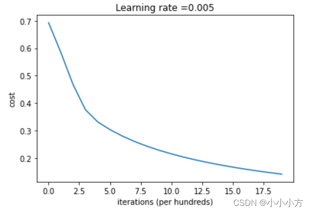

 cost下降，表明正在学习参数，可以在训练集上进一步训练模型。尝试增加单元格中的迭代次数并重新运行单元格，会看到训练集准确度上升，但测试集准确度下降，这称为过拟合。

学习率决定了参数更新的速度，学习率太大会超过最优值，太小又会需要迭代太多次才能收敛到最佳值。

learning_rates = [0.01, 0.001, 0.0001]
models = {}

for lr in learning_rates:
    print ("Training a model with learning rate: " + str(lr))
    models[str(lr)] = model(train_set_x, train_set_y, test_set_x, test_set_y, num_iterations=1500, learning_rate=lr, print_cost=False)
    print ('\n' + "-------------------------------------------------------" + '\n')

for lr in learning_rates:
    plt.plot(np.squeeze(models[str(lr)]["costs"]), label=str(models[str(lr)]["learning_rate"]))

plt.ylabel('cost')
plt.xlabel('iterations (hundreds)')

legend = plt.legend(loc='upper center', shadow=True)
frame = legend.get_frame()
frame.set_facecolor('0.90')
plt.show()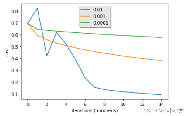

 

my_image = "my_image.jpg"   

# We preprocess the image to fit your algorithm.
fname = "images/" + my_image
image = np.array(Image.open(fname).resize((num_px, num_px)))
plt.imshow(image)
image = image / 255.
image = image.reshape((1, num_px * num_px * 3)).T
my_predicted_image = predict(logistic_regression_model["w"], logistic_regression_model["b"], image)

print("y = " + str(np.squeeze(my_predicted_image)) + ", your algorithm predicts a \"" + classes[int(np.squeeze(my_predicted_image)),].decode("utf-8") +  "\" picture.")

y = 0.0, your algorithm predicts a "non-cat" picture.