Underfitting and Overfitting

1---The depth of the tree

In "Measure Your Model Validation", we have learned how to measure model validation and how to calculate it.In this chapter, we're going to make two things clear: Underfitting and Overfitting
In the previous chapter "Improving the Decision Tree", I introduced two types of decision trees, but there are many more types. We only need to know that the most important option determines the depth of the tree.

2---Overfitting

In practice, it is not uncommon for a tree on the top floor to have 10 leaves and a leaf with 10 branches. In order for the model to predict the most accurate house price, we tend to divide the houses in a dataset into many leaves, but at the same time, each leaf corresponds to fewer and fewer houses (after all, every time we make a branch, it is a 2 squared). Yes, you did it,you predicted the most accurate house price  in the training dataset.🤣🤣🤣

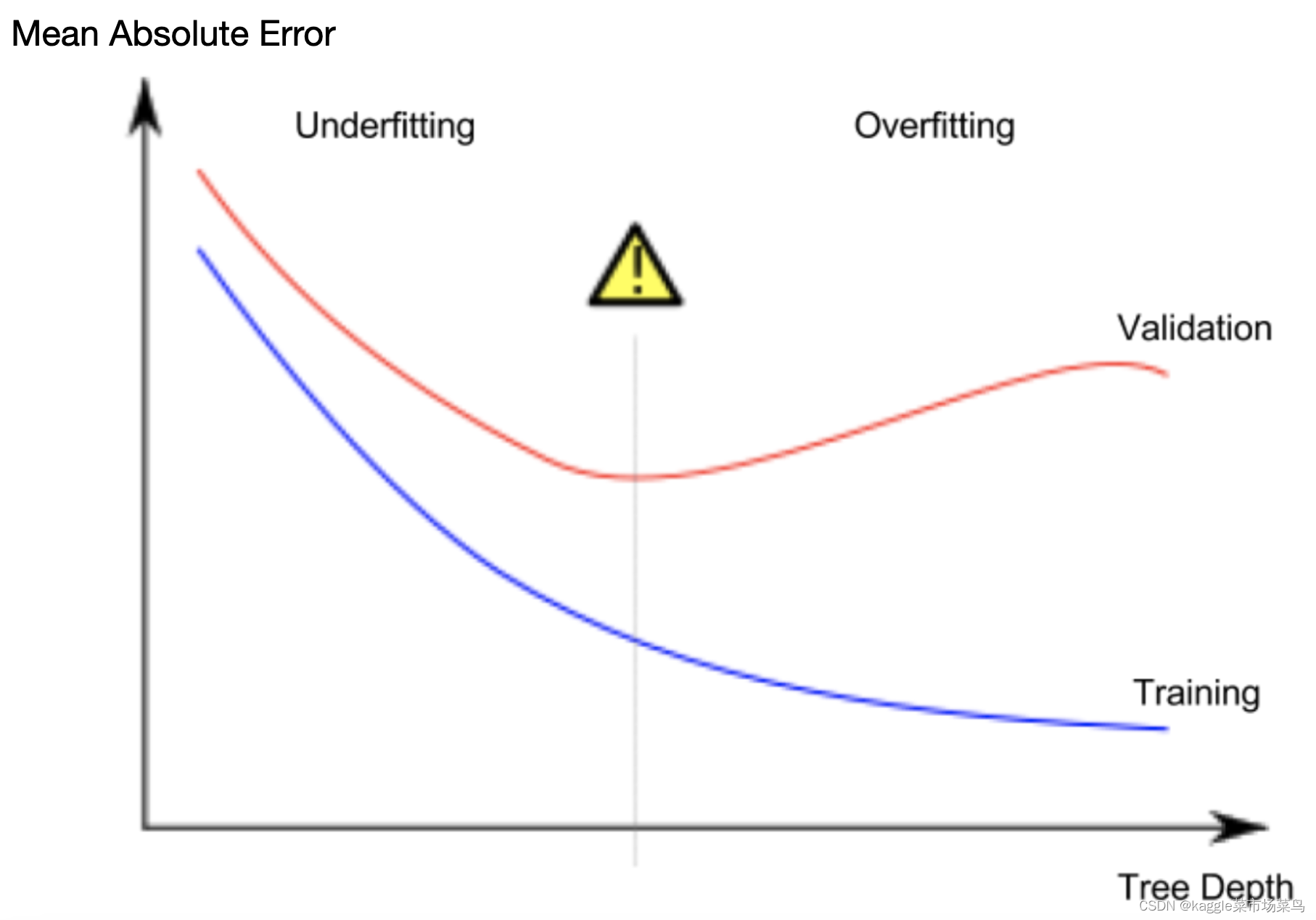
This is overfitting, which matches the training data almost perfectly, but it may not be reliable when predicting new data.

3---Underfitting

It can be understood as an invalid model. Just take out the leaf mentioned above👆🏻👆🏻 as the top layer of the decision tree,😂 and the result will be obvious: the prediction results have little to do with most houses, this model does not grasp the important differences and patterns in the training data set, 😅and the results will not be very good wherever the model is placed.

Now that the concepts are clearly distinguished, back to the validity of the model, how to find a balance between overfitting and not fitting?🥲

4---"max_leaf_nodes"

1.We can use a utility function to help compare MAE scores from different values for max_leaf_nodes.

2.We can use a for-loop to compare the accuracy of models built with different values for max_leaf_nodes.

from sklearn.metrics import mean_absolute_error
from sklearn.tree import DecisionTreeRegressor

def get_mae(max_leaf_nodes, train_X, val_X, train_y, val_y):
    model = DecisionTreeRegressor(max_leaf_nodes=max_leaf_nodes, random_state=0)
    model.fit(train_X, train_y)
    preds_val = model.predict(val_X)
    mae = mean_absolute_error(val_y, preds_val)
    return(mae)
# Data Loading Code Runs At This Point
import pandas as pd
    
# Load data
melbourne_file_path = '/Users/mac/Desktop/melb_data.csv'
melbourne_data = pd.read_csv(melbourne_file_path) 
# Filter rows with missing values
filtered_melbourne_data = melbourne_data.dropna(axis=0)
# Choose target and features
y = filtered_melbourne_data.Price
melbourne_features = ['Rooms', 'Bathroom', 'Landsize', 'BuildingArea', 
                        'YearBuilt', 'Lattitude', 'Longtitude']
X = filtered_melbourne_data[melbourne_features]

from sklearn.model_selection import train_test_split

# split data into training and validation data, for both features and target
train_X, val_X, train_y, val_y = train_test_split(X, y,random_state = 0)
# compare MAE with differing values of max_leaf_nodes
for max_leaf_nodes in [5, 50, 500, 5000]:
    my_mae = get_mae(max_leaf_nodes, train_X, val_X, train_y, val_y)
    print("Max leaf nodes: %d  \t\t Mean Absolute Error:  %d" %(max_leaf_nodes, my_mae))

runcell(0, '/Users/mac/Desktop/untitled6.py')
Max leaf nodes: 5  		 Mean Absolute Error:  347380
Max leaf nodes: 50  		 Mean Absolute Error:  258171
Max leaf nodes: 500  		 Mean Absolute Error:  243495
Max leaf nodes: 5000  		 Mean Absolute Error:  254983

5---Analysis&Conclusion

Of the options listed, 500 is the optimal number of leaves.

Overfitting: Capturing spurious patterns that won't recur in the future, leading to less accurate predictions.

Underfitting: Failing to capture relevant patterns, again leading to less accurate predictions. 

We use validation data, which isn't used in model training, to measure a candidate model's accuracy. This lets us try many candidate models and keep the best one.