AI竞赛5-Kaggle实战之信用卡反欺诈

阿值学长

已于 2023-05-26 22:49:25 修改

阅读量972

点赞数 1

分类专栏： AI竞赛文章标签：人工智能机器学习 sklearn python 分类

于 2023-05-26 22:22:48 首次发布

本文链接：https://blog.csdn.net/weixin_60536251/article/details/130894619

版权

AI竞赛专栏收录该内容

6 篇文章 5 订阅

订阅专栏

AI竞赛5-Kaggle实战之信用卡反欺诈

1.项目介绍
2.项目分析
3.数据预处理
4.特征工程
5.模型训练
6.模型评估及优化

1.项目介绍

1.1项目需求

本项目通过利用信用卡的历史交易数据，进行机器学习，构建信用卡反欺诈预测模型，提前发现客户信用卡被盗刷的事件

1.2 项目思路

在这里插入图片描述

1.3 项目背景

数据集包含由欧洲持卡人于2013年9月使用信用卡进行交的数据。此数据集显示两天内发生的交易，其中284,807笔交易中有492笔被盗刷。数据集非常不平衡，积极的类(被盗刷)占所有交易的0.172％。
它只包含作为PCA转换结果的数字输入变量。不幸的是，由于保密问题，我们无法提供有关数据的原始功能和更多背景信息。特征V1，V2，…V28是使用PCA获得的主要组件，没有用PCA转换的唯一特征是“时间”和“量”。特征’时间’包含数据集中每个事务和第一个事务之间经过的秒数。特征“金额”是交易金额，此特征可用于实例依赖的成本认知学习。特征’类’是响应变量，如果发生被盗刷，则取值1否则为0

2.项目分析

2.1 算法选择

数据是持卡人两天内的信用卡交易数据，这份数据包含很多维度，要解决的问题是预测持卡人是否会发生信用卡被盗刷。信用卡持卡人是否会发生被盗刷只有两种可能，发生被盗刷或不发生被盗刷。又因为这份数据是打标好的(字段Class是目标列)，也就是说它是一个监督学习的场景。于是判定信用卡持卡人是否会发生被盗刷是一个二元分类问题，意味着可以通过二分类相关的算法来找到具体的解决办法，本项目选用的算法是逻辑斯蒂回归(Logistic Regression)

2.2 数据分析

数据是结构化数据，不需要做特征抽象(是针对有序和无序的文本分类型特征，采用不同的方法进行处理，将其类别属性数值化)。特征V1至V28是经过PCA处理，而特征Time和Amount的数据规格与其他特征差别较大，需要对其做特征缩放，将特征缩放至同一个规格。在数据质量方面没有出现乱码或空字符的数据，可确定字段Class为标签列其他列为特征列

2.3 模型评估

这份数据是全部打标好的数据，可通过交叉验证的方法对训练集生成的模型进行评估。80%数据进行训练，20%数据进行预测和评估

2.4 项目分析总结

(1) 根据历史记录数据学习并对信用卡持卡人是否会发生被盗刷进行预测，二分类监督学习场景，选择逻辑斯蒂回归(Logistic Regression)算法
(2) 数据为结构化数据，不需要做特征抽象但需要做特征缩放

3.数据预处理

3.1 数据加载

import numpy as np
import pandas as pd
pd.set_option('display.float_format',lambda x :'%.4f' % x)
import matplotlib.pyplot as plt
import matplotlib.gridspec as gridspec
import seaborn as sns
import missingno as msno          # pip install missingno 可视化工具
from sklearn.linear_model import LogisticRegression
from sklearn.ensemble import RandomForestClassifier
from sklearn.model_selection import GridSearchCV
from sklearn.model_selection import train_test_split
from sklearn.metrics import auc,roc_auc_score,roc_curve,recall_score,accuracy_score,classification_report
from sklearn.preprocessing import StandardScaler
import warnings
warnings.filterwarnings('ignore')
from matplotlib import font_manager

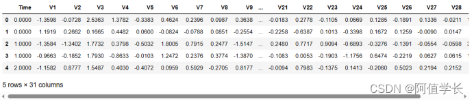
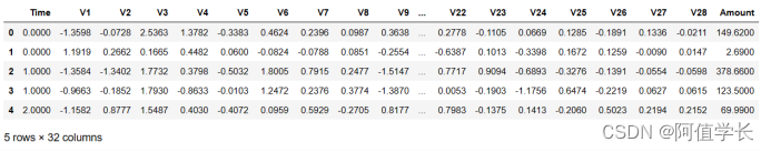
data = pd.read_csv('./creditcard.csv')
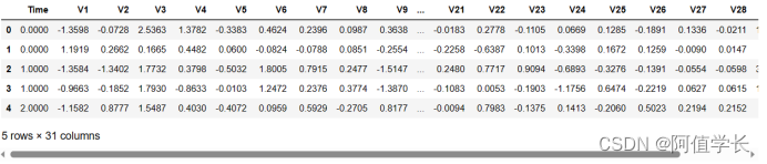
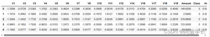
data.head()

在这里插入图片描述

3.2 数据查看

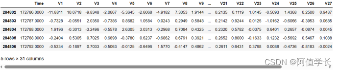
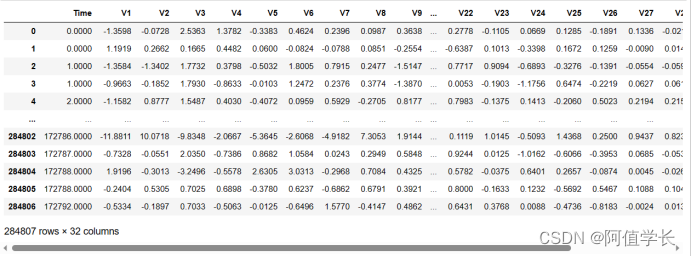
data.tail()

在这里插入图片描述

print(data.shape)
data.info()
(284807, 31)
<class 'pandas.core.frame.DataFrame'>
RangeIndex: 284807 entries, 0 to 284806
Data columns (total 31 columns):
 #   Column  Non-Null Count   Dtype  
---  ------  --------------   -----  
 0   Time    284807 non-null  float64
 1   V1      284807 non-null  float64
 2   V2      284807 non-null  float64
...
 29  Amount  284807 non-null  float64
 30  Class   284807 non-null  int64  
dtypes: float64(30), int64(1)
memory usage: 67.4 MB

3.3 统计信息查看

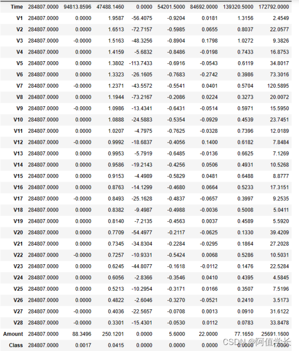
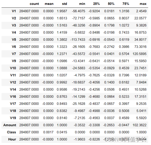
data.describe().T   # 查看数据基本统计信息 查看数据可知，时间和金额数据相对于其他特征偏大

在这里插入图片描述

3.4 缺失值查看

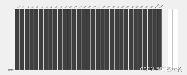
msno.matrix(data)  #  数据集不存在缺失值，因此不需作缺失值处理

在这里插入图片描述

data.isnull().sum().sum()
0

4.特征工程

4.1 标签分析

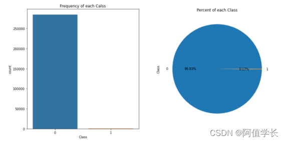
fig,axs = plt.subplots(1,2,figsize = (14,7))   
sns.countplot(x = 'Class',data = data,ax = axs[0])
axs[0].set_title('Frequency of each Calss')
data['Class'].value_counts().plot(kind = 'pie',ax = axs[1],autopct = '%1.2f%%')
axs[1].set_title('Percent of each Class')
 Text(0.5, 1.0, 'Percent of each Class')

在这里插入图片描述

 data.groupby('Class').size()  # 标签样本不均衡
Class 
0 284315 
1 492 
dtype: int64 

# 数据集284807笔交易中有492笔是信用卡被盗刷交易，信用卡被盗刷交易占总体比例为0.17%，信用卡交易正常和被盗刷两者数量不平衡，样本不平衡影响分类器的学习，稍后将会使用过采样的方法解决样本不平衡的问题

4.2 特征衍生

4.2.1 时间特征

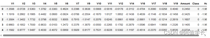
data.head()    # 时间以秒为单位，离散性太强 将其转化为以小时为单位对应每天的时间

在这里插入图片描述

data['Hour'] = data['Time'].apply(lambda x : divmod(x,3600)[0])
data

在这里插入图片描述

4.3 特征选择(数据探索)

4.3.1 特征1-信用卡正常消费及被盗刷

XFraud = data.loc[data['Class'] == 1]       # 盗刷
XnonFraud = data.loc[data['Class'] == 0]    # 正常消费
correlationNonFraud = XnonFraud.loc[:,data.columns != 'Class'].corr()
mask = np.zeros_like(correlationNonFraud)
index = np.triu_indices_from(correlationNonFraud)   # 右上部分的索引
mask[index] = True                              # mask面具：0没有面具 1表示有面具
kw = {'width_ratios':[1,1,0.05],'wspace':0.2}
f,(ax1,ax2,ax3) = plt.subplots(1,3,gridspec_kw=kw,figsize = (22,9))
cmap = sns.diverging_palette(220,8,as_cmap = True)     # 一系列颜色
sns.heatmap(correlationNonFraud,ax = ax1,vmin = -1,vmax = 1,square=False,
            linewidths=0.5,mask = mask,cbar=False,cmap= cmap)
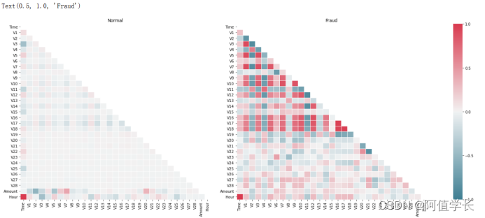
ax1.set_title('Normal')
correlationFraud = XFraud.loc[:,data.columns != 'Class'].corr()
sns.heatmap(correlationFraud,vmin = -1,vmax= 1,cmap = cmap,ax = ax2,
            square=False,linewidths=0.5,mask = mask,yticklabels=True,cbar_ax=ax3,
           cbar_kws={'orientation':'vertical','ticks':[-1,-0.5,0,0.5,1]})
ax2.set_title('Fraud')

# 从下图可以看出，信用卡被盗刷的事件中，部分变量之间的相关性更明显。其中变量V1、V2、V3、V4、V5、V6、V7、V9、V10、V11、V12、V14、V16、V17和V18以及V19之间的变化在信用卡被盗刷的样本中呈性一定的规律。特征V8、V13、V15、V20、V21、V22、V23、V24、V25、V26、V27和V28规律不明显

在这里插入图片描述

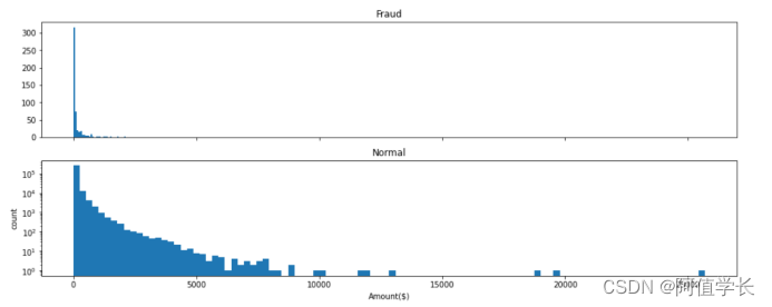
4.3.2 特征2-信用卡交易金额及交易次数

f,(ax1,ax2) = plt.subplots(2,1,sharex=True,figsize = (16,6))
ax1.hist(data['Amount'][data['Class'] == 1],bins = 30)
ax1.set_title('Fraud')
plt.yscale('log')
ax2.hist(data['Amount'][data['Class'] == 0],bins = 100)
ax2.set_title('Normal')
plt.xlabel('Amount($)')
plt.ylabel('count')
plt.yscale('log') # 信用卡被盗刷金额与正常用户金额相比呈现散而小特点，说明信用卡盗刷者更偏向选择小金额消费

在这里插入图片描述

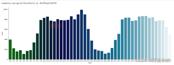
4.3.3 特征3-信用卡盗刷时间

sns.factorplot(x = 'Hour',data = data,kind = 'count',palette = 'ocean',size = 6,aspect = 3)  # size：每个面的高度(英寸)标量  aspect：纵横比标量 每天早上9点到晚上11点之间是信用卡消费的高频时间段

在这里插入图片描述

4.3.4 特征4-信用卡交易金额及交易时间

f,(ax1,ax2) = plt.subplots(2,1,sharex=True,figsize = (16,6))
cond1 = data['Class'] == 1
ax1.scatter(data['Hour'][cond1],data['Amount'][cond1])
ax1.set_title('Fraud')
cond2 = data['Class'] == 0
ax2.scatter(data['Hour'][cond2],data['Amount'][cond2])
ax2.set_title('Normal')

在这里插入图片描述

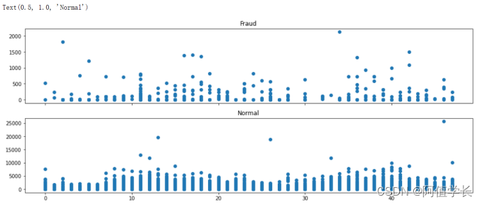
sns.catplot(x = 'Hour',kind = 'count',data = data[cond1],height=9,aspect=2)

在这里插入图片描述

data['Amount'][cond1].max()
2125.87
# 从上图可以看出，在信用卡被盗刷样本中，离群值发生在客户使用信用卡消费更低频的时间段。信用卡被盗刷数量案发最高峰在第一天上午11点达到43次，其余发生信用卡被盗刷案发时间在晚上时间11点至第二早上9点之间，说明信用卡盗刷者为了不引起信用卡卡主注意，更喜欢选择信用卡卡主睡觉时间和消费频率较高的时间点作案；同时信用卡发生被盗刷的最大值也就只有2125.87美元

4.3.5 特征分布

data.head()

在这里插入图片描述

plt.rcParams['font.family'] = 'STKaiti'
v_feat = data.iloc[:,1:29].columns
plt.figure(figsize=(16,4 * 28))
cond1 = data['Class'] == 1
cond2 = data['Class'] == 0
gs = gridspec.GridSpec(28,1)    # 子视图
for i,cn in enumerate(v_feat):
    ax = plt.subplot(gs[i])
    sns.distplot(data[cn][cond1],bins = 50)    # 欺诈
    sns.distplot(data[cn][cond2],bins = 100)   # 正常消费
    ax.set_title('特征概率分布图' + cn)
# 下图是不同变量在信用卡被盗刷和信用卡正常的不同分布情况，选择在不同信用卡状态下的分布有明显区别的变量。因此剔除变量V8、V13、V15、V20、V21、V22、V23、V24、V25、V26、V27和V28变量。这也与开始用相关性图谱观察得出结论一致。同时剔除变量Time，保留离散程度更小的Hour变量

在这里插入图片描述

4.3.6 特征删除

droplist = ['V8', 'V13', 'V15', 'V20', 'V21', 'V22', 'V23', 'V24', 'V25', 'V26', 'V27', 'V28','Time'] 
data_new = data_cr.drop(droplist, axis = 1) 
data_new.shape    # 查看数据维度 
(284807, 32)
(284807, 19)
data_new.head()  # 特征从31个缩减至18个(不含目标变量)

在这里插入图片描述

4.4 特征缩放-归一化

col = ['Amount','Hour']  # 特征Hour和Amount的量纲和其他特征相差较大，因此需对其进行特征缩放
sc = StandardScaler()     # Z-score归一化
data_new[col] = sc.fit_transform(data_new[col])
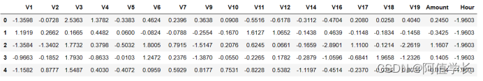
data_new.head()

在这里插入图片描述

data_new.describe().T

在这里插入图片描述

4.5 特征重要性

4.5.1 X、y变量创建
feture = list(data_new.columns)
print(feture) 
['V1', 'V2', 'V3', 'V4', 'V5', 'V6', 'V7', 'V9', 'V10', 'V11', 'V12', 'V14', 'V16', 'V17', 'V18', 'V19', 'Amount', 'Class', 'Hour']

feture.remove('Class')  # 删除特征名，修改原数据
feture
['V1',
 'V2',
 'V3',
 'V4',
 'V5',
 'V6',
 'V7',
 'V9',
 'V10',
 'V11',
 'V12',
 'V14',
 'V16',
 'V17',
 'V18',
 'V19',
 'Amount',
 'Hour']

X = data_new[feture]
y = data_new['Class']
display(X.head(),y.head())
0    0
1    0
2    0
3    0
4    0
Name: Class, dtype: int64

在这里插入图片描述

4.5.2 特征重要性排序
from sklearn.ensemble import RandomForestClassifier
clf = RandomForestClassifier()  # 利用随机森林的feature importance对特征的重要性进行排序
clf.fit(X,y)
clf.feature_importances_
array([0.01974556, 0.015216  , 0.02202158, 0.03775329, 0.01995699,
       0.02257269, 0.02873717, 0.04056692, 0.08524621, 0.06078786,
       0.18454186, 0.12167233, 0.06079882, 0.19714222, 0.03220492,
       0.01833037, 0.01716956, 0.01553564])

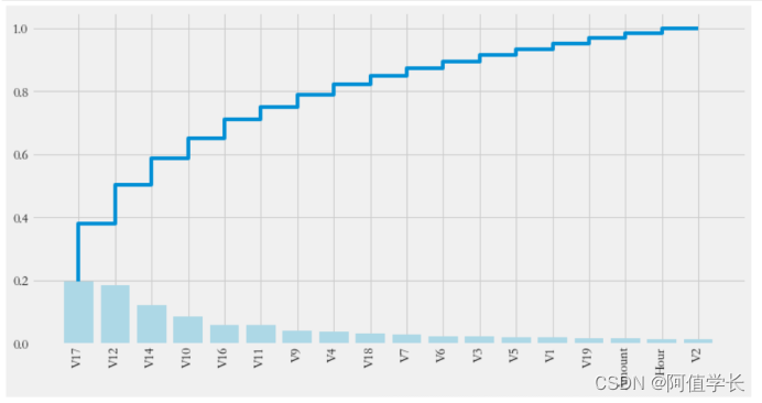
4.5.3 特征重要性显示
plt.rcParams['figure.figsize'] = (12,6)
plt.style.use('fivethirtyeight')
from matplotlib import style
style.available
['Solarize_Light2',
 '_classic_test_patch',
..
 'seaborn-whitegrid',
 'tableau-colorblind10']

 importances = clf.feature_importances_
feat_name = feture
feat_name = np.array(feat_name)
index = np.argsort(importances)[::-1]  # 特征重要性排序
plt.bar(range(len(index)),importances[index],color = 'lightblue')
plt.step(range(18),np.cumsum(importances[index]))
_ = plt.xticks(range(18),labels=feat_name[index],rotation = 'vertical',fontsize = 14)

在这里插入图片描述

5.模型训练

5.1 过采样

标签Class呈现较大的样本不平衡，会对模型学习造成困扰。样本不平衡常用的解决方法有过采样和欠采样，本项目处理样本不平衡采用的是过采样，具体操作使用SMOTE(Synthetic Minority Oversampling Technique)

# pip install imblearn
from imblearn.over_sampling import SMOTE     # 近邻规则  创造一些新数据
print('在过采样之前样本比例：\n',y.value_counts())
在过采样之前样本比例：
 0    284315
1       492
Name: Class, dtype: int64

smote = SMOTE()
X,y = smote.fit_resample(X,y)
print('在过采样之后样本比例是：\n',y)
在过采样之后样本比例是：
 0         0
1         0
         ..
568628    1
568629    1
Name: Class, Length: 568630, dtype: int64

y.value_counts()
0    284315
1    284315
Name: Class, dtype: int64

5.2 算法建模

5.2.1 准确率

model = LogisticRegression()
model.fit(X,y) # 样本是均衡的
y_ = model.predict(X)  # 信用卡反欺诈更希望算法找到盗刷的交易！ 正常交易不关心！
print('逻辑斯蒂回归算准确率是：',accuracy_score(y,y_)) 
逻辑斯蒂回归算准确率是： 0.9380581397393736

5.2.2 混淆矩阵及召回率

from sklearn.metrics import confusion_matrix    # 混淆矩阵
cm = confusion_matrix(y,y_)
print(cm)
recall = cm[1,1]/(cm[1,1] + cm[1,0])
print('召回率：',recall)
[[276963   7352]
 [ 27870 256445]]
召回率： 0.9019749221813833

def plot_confusion_matrix(cm, classes,
                          title='Confusion matrix',
                          cmap=plt.cm.Blues):
    plt.imshow(cm, interpolation='nearest', cmap=cmap)   # 混淆矩阵绘制
    plt.title(title)
    plt.colorbar()
    tick_marks = np.arange(len(classes))
    plt.xticks(tick_marks, classes, rotation=0)
    plt.yticks(tick_marks, classes)
    thresh = cm.max() / 2.
    for i, j in itertools.product(range(cm.shape[0]), range(cm.shape[1])):
        plt.text(j, i, cm[i, j],
                 horizontalalignment="center",
                 color="white" if cm[i, j] > thresh else "black")
    plt.tight_layout()
    plt.ylabel('True label')
plt.xlabel('Predicted label')
import itertools
plot_confusion_matrix(cm,classes=[0,1])

在这里插入图片描述

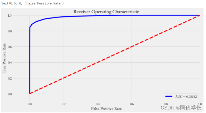
5.2.3 ROC及AUC

proba_ = model.predict_proba(X)[:,1]   # 索引1表示获取类别1的概率，正样本、阳性、信用卡盗刷
fpr,tpr,thesholds_ = roc_curve(y,proba_)  # ROC曲线(真实值,预测值)
roc_auc = auc(fpr,tpr)                  # ROC曲线下面积
plt.title('Receiver Operating Characteristic')   # ROC曲线绘制
plt.plot(fpr, tpr, 'b',label='AUC = %0.5f'% roc_auc)
plt.legend(loc='lower right')
plt.plot([0,1],[0,1],'r--')
plt.xlim([-0.1,1.0])
plt.ylim([-0.1,1.01])
plt.ylabel('True Positive Rate')
plt.xlabel('False Positive Rate')

在这里插入图片描述

6.模型评估及优化

上一个步骤中模型训练和测试都在同一个数据集上进行，这样导致模型产生过拟合的问题。一般将数据集划分为训练集和测试集有3种处理方法：
(1) 留出法(hold-out)
(2) 交叉验证法(cross-validation)
(3) 自助法(bootstrapping)
本次项目采用的是交叉验证法划分数据集，将数据划分为3部分：训练集(trainingset)、验证集(validationset)和测试集(testset)。让模型在训练集进行学习，在验证集上进行参数调优，最后使用测试集数据评估模型的性能。模型调优采用网格搜索调优参数(grid search)，通过构建参数候选集合然后网格搜索会穷举各种参数组合，根据评分机制找到最好的那一组设置。结合cross-validation和grid search，采用scikitlearn模块model_selection中的Grid SearchCV方法

6.1 交叉验证

6.1.1 模型训练
X_train, X_test, y_train, y_test = train_test_split(X, y, test_size = 0.2)
param_grid = {'C': [0.01,0.1, 1, 10, 100, 1000,],'penalty': [ 'l1', 'l2']}    # 构建网格参数
grid_search = GridSearchCV(LogisticRegression(),param_grid,cv=10)  # 模型和参数组合param_grid 、cv：10折
grid_search.fit(X_train, y_train) # 用训练集网格交叉训练算法
GridSearchCV(cv=10, estimator=LogisticRegression(),
             param_grid={'C': [0.01, 0.1, 1, 10, 100, 1000],
                         'penalty': ['l1', 'l2']})

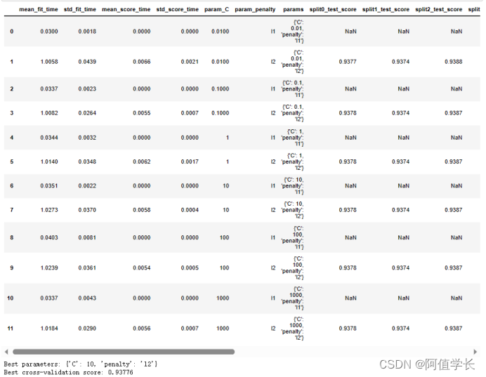
6.1.2 最佳参数查看
results = pd.DataFrame(grid_search.cv_results_) # 网格交叉结果数据格式转换
display(results)
print("Best parameters: {}".format(grid_search.best_params_))
print("Best cross-validation score: {:.5f}".format(grid_search.best_score_))

在这里插入图片描述

6.1.3 预测
y_pred = grid_search.predict(X_test)
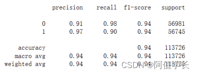
print('准确率：',accuracy_score(y_test,y_pred)) 
准确率： 0.9391432038408104

6.1.4 分类评估报告
from sklearn.metrics import classification_report
print(classification_report(y_test,y_pred))

在这里插入图片描述

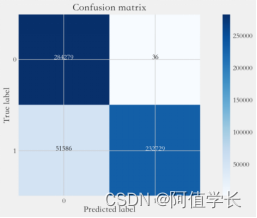
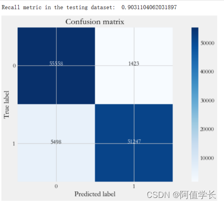
6.2 混淆矩阵

cnf_matrix = confusion_matrix(y_test, y_pred) # 生成测试数据混淆矩阵
np.set_printoptions(precision=2)   # 设置打印选项 精度为2
print("Recall metric in the testing dataset: ", cnf_matrix[1,1]/(cnf_matrix[1,0]+cnf_matrix[1,1]))
class_names = [0,1]  # 绘制模型优化后的混淆矩阵
plt.figure()
plot_confusion_matrix(cnf_matrix, classes=class_names, title='Confusion matrix')

在这里插入图片描述

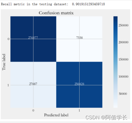
y_ = grid_search.predict(X)  # 生成全部数据混淆矩阵 最佳参数C：10、pentaly：l2
cnf_matrix = confusion_matrix(y, y_)
np.set_printoptions(precision=2)
print("Recall metric in the testing dataset: ", cnf_matrix[1,1]/(cnf_matrix[1,0]+cnf_matrix[1,1]))
class_names = [0,1]  # 绘制模型优化后的混淆矩阵
plt.figure()
plot_confusion_matrix(cnf_matrix, classes=class_names, title='Confusion matrix')
# 经过交叉验证训练和参数调优后，模型性能有较大提升，recall值从0.818上升到0.9318，上升幅度达到11.34%

在这里插入图片描述

6.3 模型评估

解决不同的问题，通常需要不同的指标来度量模型的性能。例如希望用算法来预测癌症是否是恶性的，假设100个病人中有5个病人的癌症是恶性，对于医生来说，尽可能提高模型的查全率(recall)比提高查准率(precision)更为重要，因为站在病人的角度，发生漏发现癌症为恶性比发生误判为癌症是恶性更为严重。

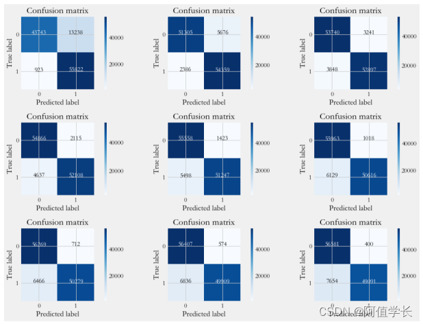
6.3.1 混淆矩阵

y_pred_proba = grid_search.predict_proba(X_test)   # 获得预测概率值
thresholds = [0.1,0.2,0.3,0.4,0.5,0.6,0.7,0.8,0.9]  # 设定不同阈值
plt.figure(figsize=(15,10))
np.set_printoptions(precision=2)
j = 1
for t in thresholds:
    y_pred = y_pred_proba[:,1] > t             # 根据阈值转换为类别
    plt.subplot(3,3,j)
    j += 1
    cnf_matrix = confusion_matrix(y_test, y_pred)  # 计算混淆矩阵
    print("召回率是：", cnf_matrix[1,1]/(cnf_matrix[1,0]+cnf_matrix[1,1]),end = '\t')
    print('准确率是：',(cnf_matrix[0,0] + cnf_matrix[1,1])/(cnf_matrix.sum()))
    class_names = [0,1]                         # 绘制混淆矩阵
    plot_confusion_matrix(cnf_matrix, classes=class_names)
召回率是： 0.9837342497136311	准确率是： 0.8754814202557023
召回率是： 0.957952242488325	准确率是： 0.9291103177813341
召回率是： 0.9321878579610539	准确率是： 0.9376659690835869
召回率是： 0.9182835492113842	准确率是： 0.9406292316620649
召回率是： 0.9031104062031897	准确率是： 0.9391432038408104
召回率是： 0.8919904837430611	准确率是： 0.9371559713697836
召回率是： 0.8860516345052427	准确率是： 0.9368833863848196
召回率是： 0.8795312362322671	准确率是： 0.9348433955296063
召回率是： 0.8651158692395806	准确率是： 0.9291806622935829

在这里插入图片描述

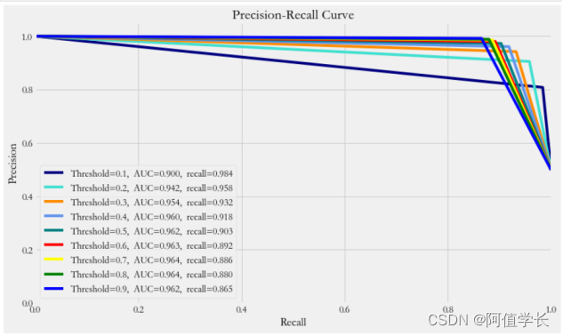
6.3.2 精确率-召回率曲线

from sklearn.metrics import precision_recall_curve
thresholds = [0.1,0.2,0.3,0.4,0.5,0.6,0.7,0.8,0.9]
colors = ['navy', 'turquoise', 'darkorange', 'cornflowerblue', 'teal', 'red', 'yellow', 'green', 'blue']
plt.figure(figsize=(12,7))
j = 1
for t,color in zip(thresholds,colors):
    y_pred = y_pred_proba[:,1] > t      # 预测出来的概率值是否大于阈值  
    precision, recall, threshold = precision_recall_curve(y_test, y_pred) # 召回率
    area = auc(recall, precision)             # auc面积
    cm = confusion_matrix(y_test,y_pred)    # 混淆矩阵
    # TP/(TP + FN)
    r = cm[1,1]/(cm[1,0] + cm[1,1])  # 绘制 Precision-Recall curve
    plt.plot(recall, precision, color=color,
                 label='Threshold=%s,  AUC=%0.3f,  recall=%0.3f' %(t,area,r))
    plt.xlabel('Recall')
    plt.ylabel('Precision')
    plt.ylim([0.0, 1.05])
    plt.xlim([0.0, 1.0])
    plt.title('Precision-Recall Curve')
    plt.legend(loc="lower left")

在这里插入图片描述

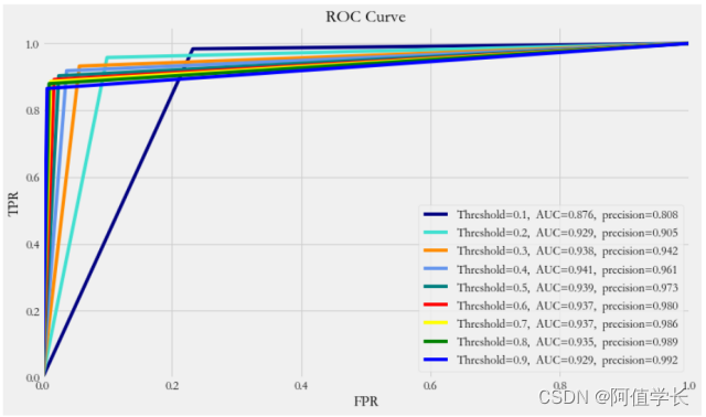
6.3.3 ROC曲线

thresholds = [0.1,0.2,0.3,0.4,0.5,0.6,0.7,0.8,0.9]
colors = ['navy', 'turquoise', 'darkorange', 'cornflowerblue', 'teal', 'red', 'yellow', 'green', 'blue']
plt.figure(figsize=(12,7))
j = 1
for t,color in zip(thresholds,colors):
#     y_pred = grid_search.predict(X_teste) 
    y_pred = y_pred_proba[:,1] >= t          # 预测出来的概率值是否大于阈值 （人为） 
    cm = confusion_matrix(y_test,y_pred)
    precision = cm[1,1]/(cm[0,1] + cm[1,1])  # TP/(TP + FP)
    fpr,tpr,_ = roc_curve(y_test,y_pred)
    accuracy = accuracy_score(y_test,y_pred)
    auc_ = auc(fpr,tpr)   # 绘制 ROC curve
    plt.plot(fpr, tpr, color=color,label='Threshold=%s,  AUC=%0.3f,  precision=%0.3f' %(t , auc_,precision)) 
    plt.xlabel('FPR')
    plt.ylabel('TPR')
    plt.ylim([0.0, 1.05])
    plt.xlim([0.0, 1.0])
    plt.title('ROC Curve')
    plt.legend(loc="lower right")

在这里插入图片描述

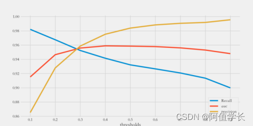
6.3.4各评估指标趋势图

'''
true negatives:`C_{0,0}`
false negatives: `C_{1,0}` 
true positives is:`C_{1,1}` 
false positives is :`C_{0,1}`
'''
thresholds = [0.1,0.2,0.3,0.4,0.5,0.6,0.7,0.8,0.9]
recalls = []      # 召回率
precisions = []   # 精确度
aucs = []        # 曲线下面积
y_pred_proba = grid_search.predict_proba(X_test)
for threshold in thresholds:
    y_ = y_pred_proba[:,1] >= threshold
    cm = confusion_matrix(y_test,y_)
    # TP/(TP + FN)   召回率：从真癌症患者中找出比例，200,85个，42.5%
    recalls.append(cm[1,1]/(cm[1,0] + cm[1,1])) 
    # TP/(TP + FP)   精确率：找到癌症患者，100个、85个真的、15个没病、预测有病
    precisions.append(cm[1,1]/(cm[0,1] + cm[1,1]))
    fpr,tpr,_ = roc_curve(y_test,y_)
    auc_ = auc(fpr,tpr)
    aucs.append(auc_)
plt.figure(figsize=(12,6))
plt.plot(thresholds,recalls,label = 'Recall')
plt.plot(thresholds,aucs,label = 'auc')
plt.plot(thresholds,precisions,label = 'precision')
plt.legend()
plt.xlabel('thresholds')

在这里插入图片描述

6.4 最优阈值

precision和recall是一组矛盾的变量。从上面混淆矩阵和PRC曲线、ROC曲线可以看到，阈值越小，recall值越大，模型能找出信用卡被盗刷的数量也就更多，但换来的代价是误判数量也较大。随着阈值的提高，recall值逐渐降低，precision值也逐渐提高，误判的数量也随之减少。通过调整模型阈值，控制模型反信用卡欺诈的力度，若想找出更多的信用卡被盗刷就设置较小的阈值，反之则设置较大的阈值。
实际业务中，阈值的选择取决于公司业务边际利润和边际成本的比较；当模型阈值设置较小的值，确实能找出更多的信用卡被盗刷的持卡人，但随着误判数量增加，不仅加大了贷后团队的工作量，也会降低误判为信用卡被盗刷客户的消费体验，从而导致客户满意度下降，如果某个模型阈值能让业务的边际利润和边际成本达到平衡时，则该模型的阈值为最优值。当然也有例外的情况，发生金融危机，往往伴随着贷款违约或信用卡被盗刷的几率会增大，而金融机构会更愿意不惜一切代价守住风险的底线。