


AI竞赛6-Kaggle实战之罗斯曼商店销量预测
1.项目介绍
- 项目目的:使用商店、促销和竞争对手数据预测销售
- Rossmann在欧洲国家经营着3000多家日化用品超市。目前,Rossmann商店经理的任务是提前6周预测他们的日销售额。商店的销售受到许多因素的影响,包括促销、竞争、学校和国家假日、季节性和地域性。由于数以千计的管理者根据自己的特殊情况预测销售,结果的准确性可能会有很大的差异。因此使用机器学习算法对销量进行预测,Rossmann要求预测德国1115家商店的6周日销售额。可靠的销售预测使商店经理能够制定有效的员工时间表,提高生产力和积极性
- 这就是算法和零售、物流领域的一次深度融合,从而提前备货,减少库存、提升资金流转率,促进公司更加健康发展,为员工更合理的工作、休息提供合理安排,为工作效率提高保驾护航

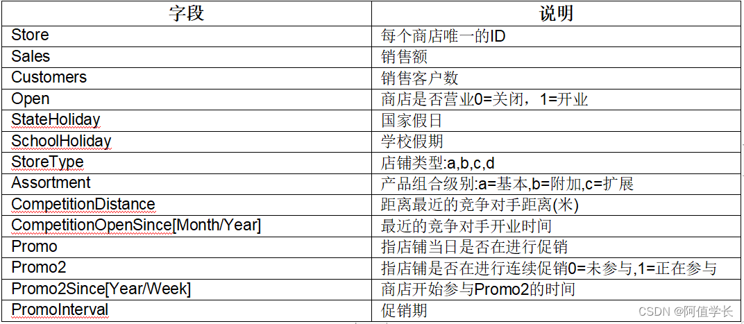
2.数据介绍
(1) train.csv:包含销售情况的历史数据文件
(2) test.csv:不包含销售情况的历史数据文件
(3) sample_submission.csv:数据提交样本文件
(4) store.csv:商店更多信息文件
(5) StateHoliday:通常所有商店都在国家假日关门:a=公共假日,b=复活节假日,c=圣诞节,0=无
3.数据加载
3.1 数据查看
import numpy as np
import pandas as pd
import matplotlib.pyplot as plt
import seaborn as sns
import xgboost as xgb
import time
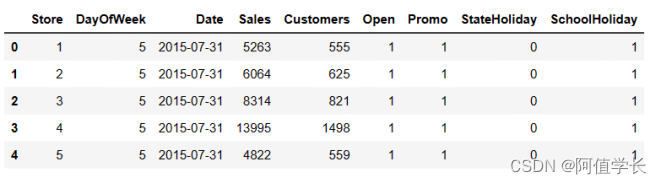
train = pd.read_csv('./data/train.csv',dtype={'StateHoliday':np.string_}) # 加载数据时为特定字段指定数据类型
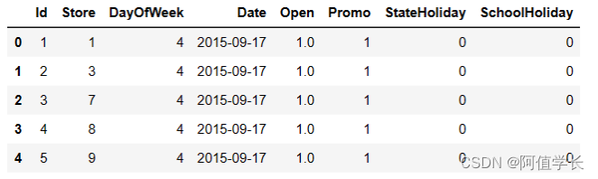
test = pd.read_csv('./data/test.csv',dtype={'StateHoliday':np.string_})
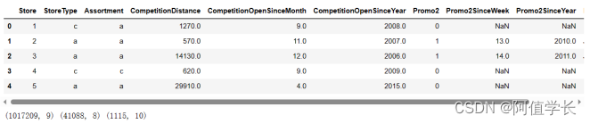
store = pd.read_csv('./data/store.csv') # 店铺详情
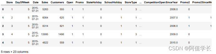
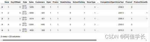
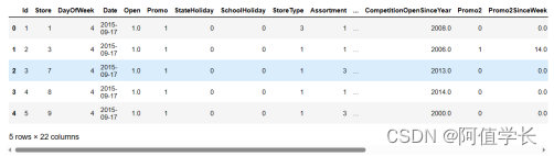
display(train.head(),test.head(),store.head()) # 数据中存在空数据,一次需要处理空数据
print(train.shape,test.shape,store.shape) # StateHoliday:a =公共假日,b =复活节假日,c =圣诞节,0 =无。既有字符串也有数字,需要指定类型
3.2 空数据处理
3.2.1 训练数据
train.isnull().sum() # 训练数据没空数据 不需要处理
Store            0
DayOfWeek        0
...
StateHoliday     0
SchoolHoliday    0
dtype: int64
3.2.2 测试数据
test.isnull().sum()
Id                0
Store             0
DayOfWeek         0
Date              0
Open             11
Promo             0
StateHoliday      0
SchoolHoliday     0
dtype: int64
cond = test['Open'].isnull()
test[cond]
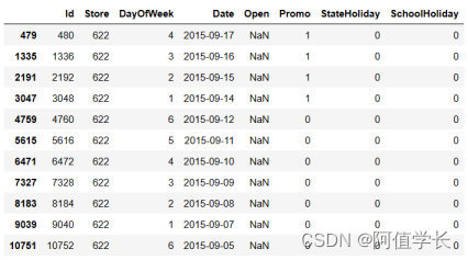
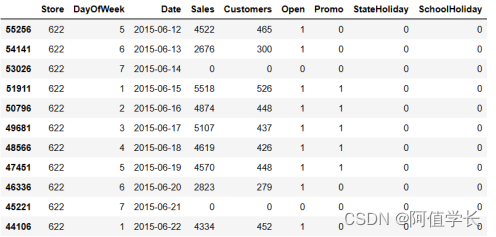
cond = train['Store'] == 622
df = train[cond]
df.sort_values(by = 'Date').iloc[-50:] # 根据过往的数据,对测试数据中622号店铺进行填充
test.fillna(1,inplace=True) # 用1填充空数据
test.isnull().sum()
Id               0
Store            0
DayOfWeek        0
Date             0
Open             0
Promo            0
StateHoliday     0
SchoolHoliday    0
dtype: int64
3.2.3 商店数据
store.isnull().sum()  # 商店缺失值较多但数量看来比较一致
Store                          0
StoreType                      0
Assortment                     0
CompetitionDistance            3
CompetitionOpenSinceMonth    354
CompetitionOpenSinceYear     354
Promo2                         0
Promo2SinceWeek              544
Promo2SinceYear              544
PromoInterval                544
dtype: int64
v1 = 'CompetitionDistance'    # 下面是观察store缺失的情况
v2 = 'CompetitionOpenSinceMonth'
v3 = 'CompetitionOpenSinceYear'
v4 = 'Promo2SinceWeek'
v5 = 'Promo2SinceYear'
v6 = 'PromoInterval'
store[(store[v2].isnull()) & (store[v3].isnull())].shape  #  v2和v3 同时缺失
(354, 10)
store[(store[v4].isnull())&(store[v5].isnull())&(store[v6].isnull())].shape  #  v4、v5、v6同时缺失
(544, 10)
# 下面对缺失数据填充   店铺竞争数据缺失而且缺失的都是对应的  原因不明而且数量也比较多,如果用中值或均值来填充有失偏颇。暂且填0解释意义就是刚开业  店铺促销信息的缺失是因为没有参加促销活动,所以以0填充
store.fillna(0,inplace=True)
store.isnull().sum()
Store                        0
StoreType                    0
Assortment                   0
CompetitionDistance          0
CompetitionOpenSinceMonth    0
CompetitionOpenSinceYear     0
Promo2                       0
Promo2SinceWeek              0
Promo2SinceYear              0
PromoInterval                0
dtype: int64
3.2.4 销量时间
  cond = train['Sales'] > 0  # 分析店铺销量随时间变化
sales_data = train[cond]   # 获取销售额为正数据
sales_data.loc[train['Store'] == 1].plot(x = 'Date',y = 'Sales',title = 'Store_1',figsize = (16,4),color = 'red')

# 从下图中可以看出店铺销售额有周期性变化,一年中11、12月份销量相对较高,可能是季节(圣诞节)因素或者促销等原因。此外从2014年6-9月份的销量来看,6、7月份的销售趋势与8、9月份类似,而需要预测的6周在2015年8、9月份,因此可以把2015年6、7月份最近6周的1115家店的数据留出作为测试数据,用于模型的优化和验证

test['Date'].unique() # 测试数据 要预测8~9月份的销售情况
array(['2015-09-17', '2015-09-16', '2015-09-15', '2015-09-14',
       '2015-09-13', '2015-09-12', '2015-09-11', '2015-09-10',
       '2015-09-09', '2015-09-08', '2015-09-07', '2015-09-06',
       '2015-09-05', '2015-09-04', '2015-09-03', '2015-09-02',
       '2015-09-01', '2015-08-31', '2015-08-30', '2015-08-29',
       '2015-08-28', '2015-08-27', '2015-08-26', '2015-08-25',
       '2015-08-24', '2015-08-23', '2015-08-22', '2015-08-21',
       '2015-08-20', '2015-08-19', '2015-08-18', '2015-08-17',
       '2015-08-16', '2015-08-15', '2015-08-14', '2015-08-13',
       '2015-08-12', '2015-08-11', '2015-08-10', '2015-08-09',
       '2015-08-08', '2015-08-07', '2015-08-06', '2015-08-05',
       '2015-08-04', '2015-08-03', '2015-08-02', '2015-08-01'],
      dtype=object)
4.合并数据
display(train.shape,test.shape)
cond = train['Sales'] > 0
train = train[cond] # 过滤销售额小于0数据
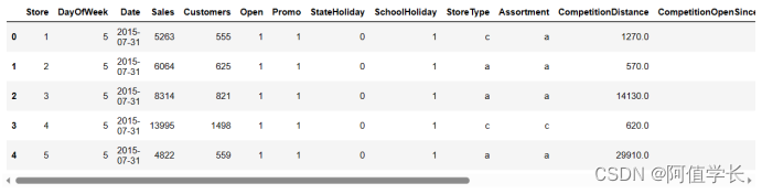
train = pd.merge(train,store,on = 'Store',how = 'left')
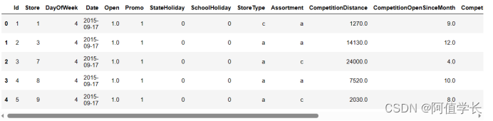
test = pd.merge(test,store,on = 'Store',how = 'left')
display(train.shape,test.shape)
(1017209, 9)
(41088, 8)
(844338, 18)
(41088, 17)
train.info()
<class 'pandas.core.frame.DataFrame'>
Int64Index: 844338 entries, 0 to 844337
Data columns (total 18 columns):
# Column Non-Null Count Dtype
--- ------ -------------- -----
0 Store 844338 non-null int64
1 DayOfWeek 844338 non-null int64
2 Date 844338 non-null object
3 Sales 844338 non-null int64
4 Customers 844338 non-null int64
5 Open 844338 non-null int64
6 Promo 844338 non-null int64
7 StateHoliday 844338 non-null object
8 SchoolHoliday 844338 non-null int64
9 StoreType 844338 non-null object
10 Assortment 844338 non-null object
11 CompetitionDistance 844338 non-null float64
12 CompetitionOpenSinceMonth 844338 non-null float64
13 CompetitionOpenSinceYear 844338 non-null float64
14 Promo2 844338 non-null int64
15 Promo2SinceWeek 844338 non-null float64
16 Promo2SinceYear 844338 non-null float64
17 PromoInterval 844338 non-null object
dtypes: float64(5), int64(8), object(5)
memory usage: 122.4+ MB
test.info()
<class 'pandas.core.frame.DataFrame'>
Int64Index: 41088 entries, 0 to 41087
Data columns (total 17 columns):
# Column Non-Null Count Dtype
--- ------ -------------- -----
0 Id 41088 non-null int64
1 Store 41088 non-null int64
2 DayOfWeek 41088 non-null int64
3 Date 41088 non-null object
4 Open 41088 non-null float64
5 Promo 41088 non-null int64
6 StateHoliday 41088 non-null object
7 SchoolHoliday 41088 non-null int64
8 StoreType 41088 non-null object
9 Assortment 41088 non-null object
10 CompetitionDistance 41088 non-null float64
11 CompetitionOpenSinceMonth 41088 non-null float64
12 CompetitionOpenSinceYear 41088 non-null float64
13 Promo2 41088 non-null int64
14 Promo2SinceWeek 41088 non-null float64
15 Promo2SinceYear 41088 non-null float64
16 PromoInterval 41088 non-null object
dtypes: float64(6), int64(6), object(5)
memory usage: 5.6+ MB
5.特征工程
train.head()
train['StateHoliday'].unique()
array(['0', 'a', 'b', 'c'], dtype=object)
test.head()
for data in [train,test]:
data['year'] = data['Date'].apply(lambda x : x.split('-')[0]).astype(int) # 时间特征拆分和转化
data['month'] = data['Date'].apply(lambda x : x.split('-')[1]).astype(int)
data['day'] = data['Date'].apply(lambda x : x.split('-')[2]).astype(int)
# PromoInterval是string类型无法建模,将其转化为IsPromoMonth:是否进行促销 1表示是
month2str = {1:'Jan',2:'Feb',3:'Mar',4:'Apr',5:'May',6:'Jun',7:'Jul',8:'Aug',9:'Sep',10:'Oct',11:'Nov',12:'Dec'}
data['monthstr'] = data['month'].map(month2str)
convert = lambda x : 0 if x['PromoInterval'] == 0 else 1 if x['monthstr'] in x['PromoInterval'] else 0 # convert 转换
data['IsPromoMonth'] = data.apply(convert,axis = 1) # 这个月是否为促销月
mappings = {'0':0,'a':1,'b':2,'c':3,'d':4} # 将字符串类型转换成数字:StoreType、Assortment、StateHoliday
data['StoreType'].replace(mappings,inplace = True)
data['Assortment'].replace(mappings,inplace = True)
data['StateHoliday'].replace(mappings,inplace = True)
train['StoreType'].unique()
array([3, 1, 4, 2], dtype=int64)
train['Assortment'].unique()
array([1, 3, 2], dtype=int64)
train['StateHoliday'].unique()
array([0, 1, 2, 3], dtype=int64)
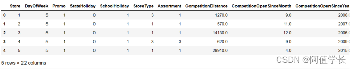
train.head()
test.info()
<class 'pandas.core.frame.DataFrame'>
Int64Index: 41088 entries, 0 to 41087
Data columns (total 22 columns):
 #   Column                     Non-Null Count  Dtype
---  ------                     --------------  -----
 0   Id                         41088 non-null  int64
 1   Store                      41088 non-null  int64
 2   DayOfWeek                  41088 non-null  int64
 3   Date                       41088 non-null  object
 4   Open                       41088 non-null  float64
 5   Promo                      41088 non-null  int64
 6   StateHoliday               41088 non-null  int64
 7   SchoolHoliday              41088 non-null  int64
 8   StoreType                  41088 non-null  int64
 9   Assortment                 41088 non-null  int64
 10  CompetitionDistance        41088 non-null  float64
 11  CompetitionOpenSinceMonth  41088 non-null  float64
 12  CompetitionOpenSinceYear   41088 non-null  float64
 13  Promo2                     41088 non-null  int64
 14  Promo2SinceWeek            41088 non-null  float64
 15  Promo2SinceYear            41088 non-null  float64
 16  PromoInterval              41088 non-null  object
 17  year                       41088 non-null  int32
 18  month                      41088 non-null  int32
 19  day                        41088 non-null  int32
 20  monthstr                   41088 non-null  object
 21  IsPromoMonth               41088 non-null  int64
dtypes: float64(6), int32(3), int64(10), object(3)
memory usage: 6.7+ MB
6.训练及测试数据
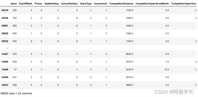
display(train.head(),test.head())
display(train.shape,test.shape)
df_train = train.drop(['Date','monthstr','PromoInterval','Customers','Open'],axis = 1)
df_test = test.drop(['Date','monthstr','PromoInterval','Open','Id'],axis = 1) # 删掉训练和测试数据集中不需要特征
display(df_train.shape,df_test.shape)
(844338, 23)
(41088, 22)
(844338, 18)
(41088, 17)
X_train = df_train[6*7*1115:]   # 建模训练数据
X_test = df_train[:6*7*1115]   # 建模验证数据(评估)  2015年6~7月份销售数据
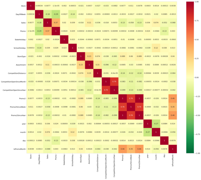
7.数据属性相关性系数
plt.figure(figsize=(24,20))
plt.rcParams['font.size'] = 12
sns.heatmap(df_train.corr(),cmap='RdYlGn_r',annot=True,vmin=-1,vmax=1)
8.训练数据集
_ = plt.hist(X_train['Sales'],bins = 100) # 目标值、销售额正态分布不够正
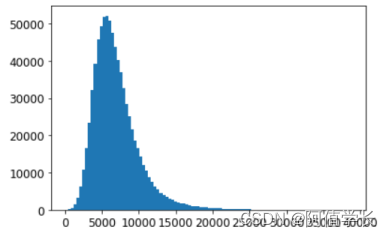
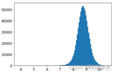
y_train = np.log1p(X_train['Sales'])
y_test = np.log1p(X_test['Sales']) # 对数化、正态化更加规整正态化
X_train = X_train.drop('Sales',axis = 1)
X_test = X_test.drop('Sales',axis = 1)
_ = plt.hist(y_train,bins = 100)
9.模型构建
9.1 评价函数
- 均方根百分比误差:

def rmspe(y,yhat):
    return np.sqrt(np.mean(1 - yhat/y)**2)
def rmspe_xg(y,yhat):    # 放大作用
    y = np.expm1(y)
    yhat = np.expm1(yhat.get_label())   # DMaxtrix数据类型  get_label获取数据
    return 'rmspe',rmspe(y,yhat)
9.2 模型训练
%%time
params = {'objective':'reg:linear',
          'booster':'gbtree',
          'eta':0.03,
          'max_depth':10,
          'subsample':0.9,
          'colsample_bytree':0.7,
          'silent':1,
          'seed':10}
num_boost_round = 6000
dtrain = xgb.DMatrix(X_train,y_train)
dtest = xgb.DMatrix(X_test,y_test)    # 保留验证数据
print('模型训练开始……')
evals = [(dtrain,'train'),(dtest,'validation')]
gbm = xgb.train(params,   # 模型参数
          dtrain,         # 训练数据
          num_boost_round,   # 轮次  决策树个数
          evals = evals,        # 验证评估数据
          early_stopping_rounds=100,    # 在验证集上当连续n次迭代,分数没有提高后提前终止训练
          feval=rmspe_xg,       # 模型评估函数
          verbose_eval=True)    # 打印输出log日志  每次训练详情
模型训练开始……
Parameters: { "silent" } might not be used.
  This may not be accurate due to some parameters are only used in language bindings but
  passed down to XGBoost core.  Or some parameters are not used but slip through this
  verification. Please open an issue if you find above cases.
[0]	train-rmse:8.01963	train-rmspe:6230.18506	validation-rmse:8.04813	validation-rmspe:6387.25244
[1]	train-rmse:7.77951	train-rmspe:4099.43457	validation-rmse:7.80813	validation-rmspe:4203.82471
...
[407]	train-rmse:0.13600	train-rmspe:0.00917	validation-rmse:0.15248	validation-rmspe:0.00460
[408]	train-rmse:0.13579	train-rmspe:0.00914	validation-rmse:0.15231	validation-rmspe:0.00462
Wall time: 2min 38s
9.2.1 params参数
(1) eta[默认0.3]:和GBM中learning rate参数类似。通过减少每一步的权重可提高模型鲁棒性。典型值:0.01-0.2
(2) max_depth[默认3]:树最大深度,这个值也是用来避免过拟合  典型值:3-10
(3) subsample[默认1]:这个参数控制对每棵树随机采样比例。减小这个参数值算法会更保守避免过拟合。但这个值设置过小可能会欠拟合。典型值:0.5-1
(4) colsample_bytree[默认1]:控制每颗树随机采样的列数占比,每一列是一个特征  0.5-1 (依据特征个数判断)
(5) seed[默认0]:随机数种子,可复现随机数据结果也可用于调整参数
(6) booster[默认是gbtree ]:选择每次迭代模型,有两种选择:gbtree基于树模型、gbliner线性模型
(7) silent[默认值0]:取0时表示打印出运行时信息,取1时表示以缄默方式运行不打印运行时信息
(8) objective[默认reg:linear]:需要被最小化损失函数。最常用值有:binary:logistic二分类逻辑回归,返回预测概率类别。multi:softmax使用softmax多分类器,返回预测类别。还要多设置一个参数:num_class类别数目
 "reg:linear": 线性回归
 "reg:logistic":逻辑回归
 "binary:logistic": 二分类的逻辑回归问题,输出为概率
 "binary:logitraw":二分类的逻辑回归问题,输出的结果为wTx
 "count:poisson":计数问题的poisson回归,输出结果为poisson分布。在poisson回归中max_delta_step的缺省值为0.7  (used to safeguard optimization)
 "multi:softmax":让XGBoost采用softmax目标函数处理多分类问题,同时需要设置参数num_class
 "multi:softprob":和softmax一样,但输出ndata * nclass向量,可将该向量reshape成ndata行nclass列矩阵。没行数据表示样本所属于每个类别概率
 "rank:pairwise":set XGBoost to do ranking task by minimizing the pairwise loss
9.2.2 train参数
(1) params:是一个字典,里面包含着训练中的参数关键字和对应的值
(2) dtrain:训练数据
(3) num_boost_round:迭代次数,也就是生成多少基模型
(4) evals:是一个列表,用于对训练过程中进行评估列表中的元素
(5) feval:自定义评估函数
(6) early_stopping_rounds:早停止次数,假设为100,验证集误差迭代到一定程度在100次内不能再继续降低就停止迭代。要求evals里至少有一个元素
(7) verbose_eval(可输入布尔型或数值型):也要求evals里至少有一个元素。如果为True则对evals中元素的评估结果会输出在结果中;如果输入数字假设为5则每隔5个迭代输出一次
(8) learning_rates:每一次提升学习率的列表
(9) xgb_model:在训练之前用于加载的xgb model
9.3 模型保存
gbm.save_model('./train_model.json')
9.4 模型评估
print('验证数据表现:')
X_test.sort_index(inplace=True)
y_test.sort_index(inplace=True)
yhat = gbm.predict(xgb.DMatrix(X_test))
error = rmspe(np.expm1(y_test),np.expm1(yhat))
print('RMSPE:',error)
验证数据表现:
RMSPE: 0.0280719416230981
res = pd.DataFrame(data = y_test)
res['Prediction'] = yhat
res = pd.merge(X_test,res,left_index=True,right_index=True)
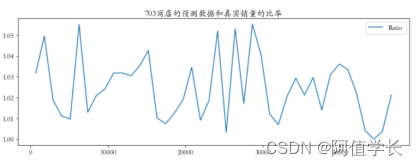
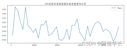
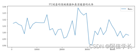
res['Ratio'] = res['Prediction']/res['Sales'] # 预测和真实销量的比率
res['Error'] = abs(1 - res['Ratio']) # 误差率
res['weight'] = res['Sales']/res['Prediction'] # 真实销量占预测值的百分比
display(res.head())
plt.rcParams['font.family'] = 'STKaiti'
col_1 = ['Sales','Prediction']
col_2 = ['Ratio']
shops = np.random.randint(1,1116,size = 3) # 随机选择三个店铺可视化
print('全部商店预测值和真实销量的比率是%0.3f' %(res['Ratio'].mean()))
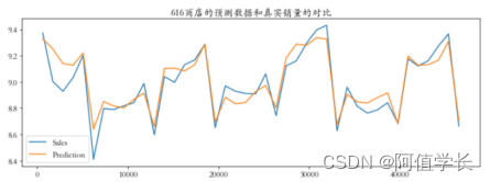
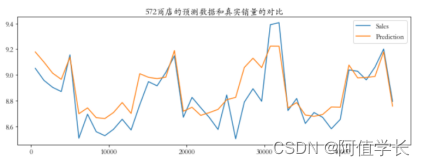
for shop in shops:
cond = res['Store'] == shop
df1 = pd.DataFrame(data = res[cond],columns = col_1)
df2 = pd.DataFrame(data = res[cond],columns = col_2)
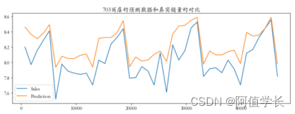
df1.plot(title = '%d商店的预测数据和真实销量的对比' % (shop),figsize = (12,4))
df2.plot(title = '%d商店的预测数据和真实销量的比率' % (shop),figsize = (12,4))
全部商店预测值和真实销量的比率是1.002
res.sort_values(by = ['Error'],ascending=False)  # 偏差数据
# 从分析结果来看,初始模型已经可以比较好的预测保留数据集的销售趋势,但相对真实值模型的预测值整体要偏高一些。从对偏差数据分析来看,偏差最大的3个数据也明显偏高。因此可以保留数据集为标准对模型进行偏差校正
9.5 模型优化
weights = [(0.99 + (i/1000)) for i in range(20)]
errors = []
for w in weights:
    error = rmspe(np.expm1(y_test),np.expm1(yhat * w)) # 偏差校正:这就是对预测值进行权重乘法 微小改变
    errors.append(error)
errors = pd.Series(errors,index=weights)
plt.figure(figsize=(9,6))
errors.plot()
plt.xlabel('权重系数',fontsize = 18)
plt.ylabel('均方根百分比误差',fontsize = 18)
index = errors.argmin()
print('最佳的偏差校正权重:',index,errors.iloc[7],weights[index])
最佳的偏差校正权重: 7 0.0013254117199704312 0.997

# 当校正系数为0.996时保留数据集的RMSPE得分最低:0.125839。相对于初始模型0.129692得分有很大的提升。因为每个店铺都有自己的特点,而设计模型对不同的店铺偏差并不完全相同,所以需要根据不同的店铺进行一个细致的校正

9.6 全局优化
shops = np.arange(1,1116)
weights1 = []   # 验证数据每个店铺的权重系数46830
weights2 = []   # 测试数据每个店铺的权重系数41088  提交到Kaggle官网
for shop in shops:
    cond = res['Store'] == shop
    df1 = pd.DataFrame(res[cond], columns=col_1) # 验证数据的预测数据和真实销量
    cond2 = df_test['Store'] == shop
    df2 = pd.DataFrame(df_test[cond2])
    weights = [(0.98 + (i/1000)) for i in range(40)]
    errors = []
    for w in weights:
        error = rmspe(np.expm1(df1['Sales']),np.expm1(df1['Prediction'] * w))
        errors.append(error)
    errors = pd.Series(errors,index = weights)
    index = errors.argmin()    # 最小索引
    best_weight = np.array(weights[index]) # 只是一个数值
    weights1.extend(best_weight.repeat(len(df1)).tolist())
    weights2.extend(best_weight.repeat(len(df2)).tolist())  # for循环结束每个店铺的权重是多少,计算得到
X_test = X_test.sort_values(by = 'Store') # 验证数据调整校正系数的排序
X_test['weights1'] = weights1    # 权重和店铺一一对应
X_test = X_test.sort_index()     # 根据索引大小排序
weights1 = X_test['weights1']
X_test = X_test.drop('weights1',axis = 1)
df_test = df_test.sort_values(by = 'Store')   # 测试数据调整校正系数
df_test['weights2'] = weights2
df_test = df_test.sort_index()
weights2 = df_test['weights2']
df_test = df_test.drop('weights2',axis = 1)
set(weights1)
{0.98,
 0.981,
...
 1.018,
 1.019}
yhat_new = yhat * weights1   # 预测销售额 校正
rmspe(np.expm1(y_test),np.expm1(yhat_new))
0.0021121179356354716
9.7 模型预测
test = xgb.DMatrix(df_test)
y_pred = gbm.predict(test)   # 算法预测结果提交Kaggle

# 初始模型
result = pd.DataFrame({'ID':np.arange(1,41089),'Sales':np.expm1(y_pred)})
result.to_csv('./result_1.csv',index=False)

# 整体校正模型
w = 0.997
result = pd.DataFrame({'ID':np.arange(1,41089),'Sales':np.expm1(y_pred * w)})
result.to_csv('./result_2.csv',index=False)

# 更细致校正模型
weights2
result = pd.DataFrame({'ID':np.arange(1,41089),'Sales':np.expm1(y_pred * weights2)})
result.to_csv('./result_3.csv',index=False)

# 上面构建的模型经过优化后已经有着不错的表现。如果想继续提高预测的精度可以在模型融合上试试


 2263
2263


 被折叠的 条评论
为什么被折叠?
被折叠的 条评论
为什么被折叠?
 到【灌水乐园】发言


