基于稀疏约束的图像去噪算法研究（Matlab代码实现）

 💥💥💞💞欢迎来到本博客❤️❤️💥💥

🏆博主优势：🌞🌞🌞博客内容尽量做到思维缜密，逻辑清晰，为了方便读者。

⛳️座右铭：行百里者，半于九十。

目录

💥1 概述

📚2 运行结果

🎉3 参考文献

🌈4 Matlab代码实现

💥1 概述

图像数据在人们日常的沟通和交流中不可或缺,然而图像在传输和接收等过程中,往往会因为硬件设备等原因受到噪声的干扰,这会降低图像的质量,并影响后续对图像的处理与分析。因此,去除图像噪声至关重要。目前,如何在去除噪声的同时保护图像的纹理细节仍是亟待解决的问题。近年来,稀疏表示理论的兴起使图像去噪取得了较大的突破。

基于稀疏约束的图像去噪算法

1. **稀疏表示理论**：稀疏表示理论是图像去噪的基础。它假设图像可以在某种变换域（如小波变换、傅里叶变换或字典学习）中用少量非零系数表示。通过找到这些稀疏表示，可以有效地去除噪声。

2. **字典学习**：字典学习是一种重要的稀疏表示方法。它通过从大量的图像块中学习一个冗余字典，使得每个图像块可以用该字典中的少量原子表示。常见的字典学习算法包括K-SVD和MOD。

3. **正则化技术**：在稀疏约束的图像去噪中，常见的正则化技术包括L1范数正则化和总变差（TV）正则化。L1范数正则化鼓励解的稀疏性，而总变差正则化则能保持图像的边缘和纹理细节。

 典型的基于稀疏约束的图像去噪算法

1. **K-SVD算法**：K-SVD算法是一种基于字典学习的稀疏表示方法。它通过交替优化字典和稀疏表示，逐步逼近最优解。在去噪过程中，K-SVD算法首先从噪声图像中提取图像块，然后利用字典学习得到稀疏表示，再通过重构得到去噪后的图像。

2. **BM3D算法**：BM3D（Block-Matching and 3D Filtering）算法结合了块匹配和三维变换技术，通过将相似的图像块堆叠成三维数组，在变换域中进行硬阈值处理，再通过逆变换和加权平均重构图像。BM3D在去噪效果和计算效率上具有很好的平衡。

3. **LASSO（Least Absolute Shrinkage and Selection Operator）**：LASSO是一种基于L1范数正则化的稀疏编码方法。它通过求解带有L1正则化的最小二乘问题，实现图像去噪。在实际应用中，LASSO通常与其他算法结合使用，以提高去噪效果。

研究现状与发展方向

1. **深度学习与稀疏表示的结合**：近年来，深度学习在图像处理领域取得了显著进展。结合深度学习和稀疏表示，可以进一步提高图像去噪的效果。例如，卷积神经网络（CNN）可以自动学习图像的稀疏表示，并用于去噪任务。

2. **自适应稀疏表示**：传统的稀疏表示方法通常依赖于预先定义的字典或变换。自适应稀疏表示通过在线学习或自适应调整字典，可以更好地适应不同类型的噪声和图像特征，提高去噪效果。

3. **多尺度稀疏表示**：多尺度方法通过在不同尺度上进行稀疏表示，可以更全面地捕捉图像的细节和结构信息，提高去噪效果。

4. **实时与高效算法**：随着图像分辨率的提高和应用场景的复杂化，开发实时和高效的图像去噪算法变得越来越重要。结合GPU加速和并行计算技术，可以显著提高算法的执行速度。

基于稀疏约束的图像去噪算法在理论研究和实际应用中都具有重要意义。随着技术的发展，这一领域将继续涌现出新的算法和方法，为图像处理带来更多的创新和进步。

📚2 运行结果

 部分代码：

pathname        = uigetdir;
allfiles        = dir(fullfile(pathname,'*.jpg'));
xts=[];         % initialize testing inputs
for i=1:size(allfiles,1)    
x=imread([pathname '\\' allfiles(i).name]);
x=imresize(x,gamma);
x=rgb2gray(x);
x=double(x);
xts=[xts; x];% testing set building
end

%% Initialization of the Algorithm
NumberofHiddenNeurons=500;  % number of neurons
D_ratio=0.35;               % the ratio of noise in each chosen frame
DB=1;                       % the power of white gaussian noise in decibels 
ActivationFunction='sig';   % Activation function
frame=20;                   % size of each frame
%% Train and test
%%
% 
%  During training, gaussian white noise and zeros will be added to 
%  randomly chosen frames .
%  The Autoencoder will be trained to avoide this type of data corruption.

[AE_net]=elm_AE(xtr,xts,NumberofHiddenNeurons,ActivationFunction,D_ratio,DB,frame)
%% Important Note: 
%%
% 
%  After completing the training process,we will no longer in need  To use 
%  InputWeight for mapping the inputs to the hidden layer, and  instead of 
%  that we will use the Outputweights beta  for coding and decoding phases
%  and also we can't use the activation  functon because  beta  is coputed 
%  after the activation .
%  The same thing is applied on biases (please for more details check the 
%  function'ELM_AE' at the testing phase).

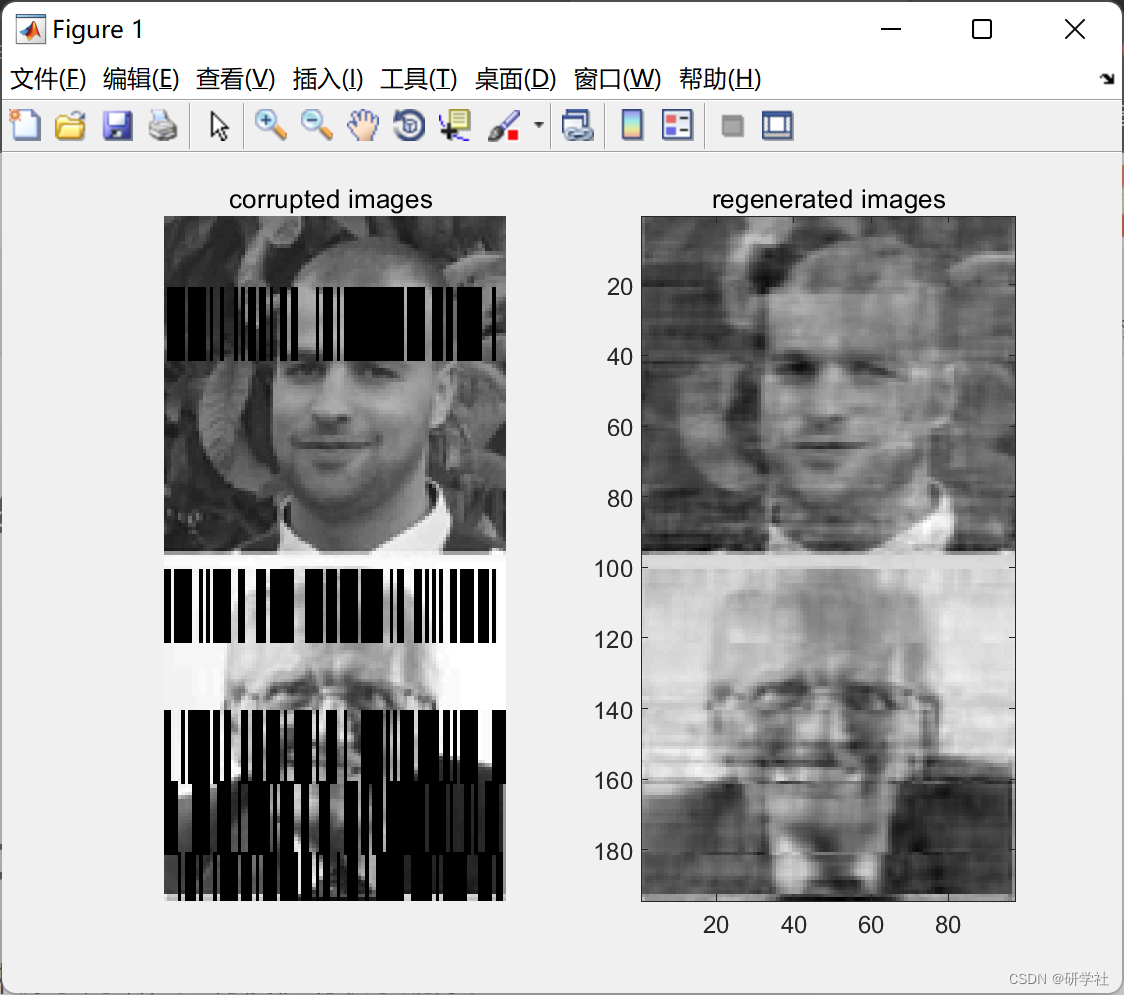
%% Illustration
subplot(121)
corrupted=AE_net.x(:,1:gamma(2)*2);
imshow(corrupted')
title('corrupted images ');
subplot(122)
regenerated=AE_net.Ytr_hat(:,1:gamma(2)*2);
imagesc(regenerated'), colormap('gray');
title('regenerated images');

%% scale training dataset
T=Tinputs';T = scaledata(T,0,1);% memorize originale copy of the input and use it as a target
P=Tinputs';
%% scale training dataset
TV.T=Tsinputs';TV.T = scaledata(TV.T,0,1);% memorize originale copy of the input and use it as a target
TV.P=Tsinputs';TV.P = scaledata(TV.P,0,1);% temporal input
TVT=TV.T;%save acopy as an output of the function

%% in the 1st and 2nd step we will corrupte the temporal input
PtNoise=zeros(size(P));
i=1;
while i < size(P,2)-frame
gen=randi([0,1],1,1);
PNoise=[];

%%% 1st step: generate set of indexes to set some input's values to zero later 
%%% (here we set them randomly and you can choose them by probability)%%%
[zeroind] = dividerand(size(P,1),1-D_ratio,0,D_ratio);% generate indexes
%%% 2nd step: add gaussian noise 
if gen==1
Noise=wgn(1,size(P,1),DB)';% generate white gaussian noise
else
Noise=zeros(1,size(P,1))'; 
end

for j=1:frame;%copy  noise
PNoise=[PNoise Noise];
end
if gen==1
for j=1:length(zeroind);% set to zero
    PNoise(zeroind(j),:)=0;
    P(zeroind(j),i:i+frame)=0;
end
end

PtNoise(:,i:i+frame-1)=PNoise;
i=i+frame;
end
 

🎉3 参考文献

部分理论来源于网络，如有侵权请联系删除。

[1]P. Vincent, H. Larochelle, I. Lajoie, Y. Bengio, and P.-A. Manzagol, “Stacked Denoising Autoencoders: Learning Useful Representations in a Deep Network with a Local Denoising Criterion,” J. Mach. Learn. Res., vol. 11, no. 3, pp. 3371–3408, 2010.
[2]L. le Cao, W. bing Huang, and F. chun Sun, “Building feature space of extreme learning machine with sparse denoising stacked-autoencoder,” Neurocomputing, vol. 174, pp. 60–71, 2016.
[3]G. Bin Huang, “What are Extreme Learning Machines? Filling the Gap Between Frank Rosenblatt’s Dream and John von Neumann’s Puzzle,” Cognit. Comput., vol. 7, no. 3, pp. 263–278, 2015.

🌈4 Matlab代码实现