【读论文】Periodic Vibration Gaussian: Dynamic Urban Scene Reconstruction and Real-time Rendering

1. What

What kind of thing is this article going to do (from the abstract and conclusion, try to summarize it in one sentence)

Utilizing periodic vibration-based temporal dynamics to represent the characteristics of various objects and elements in dynamic urban scenes. A novel temporal smoothing mechanism and a position-aware adaptive control strategy were also introduced to handle temporally coherent. Finish the reconstruction of dynamic scenes.

2. Why

Under what conditions or needs this research plan was proposed (Intro), what problems/deficiencies should be solved at the core, what others have done, and what are the innovation points? (From Introduction and related work)

Maybe contain Background, Question, Others, Innovation:

Introduction:

1. NSG: Decomposes dynamic scenes into scene graphs
2. PNF: Decomposes scenes into objects and backgrounds, incorporating a panoptic segmentation auxiliary task.
3. SUDS: Use optical flow(Optical flow helps in identifying which parts of the scene are static and which are dynamic)
4. EmerNeRF: Use a self-supervised method to reduce dependence on optical flow.

Related work:

1. Dynamic scene models
   • In one research direction, certain studies [2, 7, 11, 18, 38] introduce time as an additional input to the radiance field, treating the scene as a 6D plenoptic function. However, this approach couples positional variations induced by temporal dynamics with the radiance field, lacking geometric priors about how time influences the scene.
   • An alternative approach [1, 20, 24–26, 33, 40] focuses on modeling the movement or deformation of specific static structures, assuming that the dynamics arise from these static elements within the scene.
   • Gaussian-based
2. Urban scene reconstruction

• One research avenue(NeRF-based) has focused on enhancing the modeling of static street scenes by utilizing scalable representations [19, 28, 32, 34], achieving high-fidelity surface reconstruction [14, 28, 39], and incorporating multi-object composition [43]. However, these methods face difficulties in handling dynamic elements commonly encountered in autonomous driving contexts.
• Another research direction seeks to address these challenges. Notably, these techniques require additional input, such as leveraging panoptic segmentation to refine the dynamics of reconstruction [PNF]. [Street Gaussians, Driving Gaussian] decompose the scene with different sets of Gaussian points by bounding boxes. However, they all need manually annotated or predicted bounding boxes and have difficulty reconstructing the non-rigid objects.

3. How

The input data contain images, represented as { I i , t i , E i , I i ∣ i = 1 , 2 , … N c } \{\mathcal{I}_{i},t_{i},\mathbf{E}_{i},\mathbf{I}_{i}|i=1,2,\ldots N_{c}\} {Ii​,ti​,Ei​,Ii​∣i=1,2,…Nc​} and LiDAR point clouds represented as $\{(x_i,y_i,z_i,t_i)|i=1,2,\dots N_l\}$. The rendering process can be represented as $\hat{\mathcal{I}}={\mathcal{F}}_{\theta }({\mathbf{E}}_o,{\mathbf{I}}_o,t)$, which shows the image at any timestamp $t$ and camera pose $({\mathbf{E}}_o,{\mathbf{I}}_o)$.

3.1 PVG

The motivation behind this concept is to assign a distinct lifespan to each Gaussian
point, defining when it actively contributes and to what degree.

1. Overall pipeline:
   

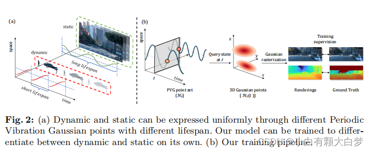
2. Mathematically,
   The Gaussian model can be denoted as H ( t ) = { μ ~ ( t ) , q , s , o ~ ( t ) , c } , \mathcal H(t)=\{\widetilde{\boldsymbol\mu}(t),\boldsymbol q,\boldsymbol s,\widetilde o(t),\boldsymbol c\}, H(t)={μ ​(t),q,s,o (t),c}, where,
   $$\begin{array}{rl}\tilde{\mathbf{\mu }}(t)& =\mathbf{\mu }+\frac{l}{2\pi }\cdot \sin (\frac{2\pi (t-\tau )}{l})\cdot \mathbf{v}\\ \tilde{o}(t)& =o\cdot e^{-\frac{1}{2}(t-\tau {)}^2{\beta }^{-2}}.\end{array}$$
   These told me how the mean value and opacity change over time. And we list the parameters that need to be learned:
   { μ , q , s , o , c , τ , β , v } ， \{\boldsymbol{\mu},\boldsymbol{q},\boldsymbol{s},o,\boldsymbol{c},\tau,\beta,\boldsymbol{v}\}， {μ,q,s,o,c,τ,β,v}，
   where $\tau$ is the life span and $\mathbf{v}$ is the velocity, indicating the direction and value at time $t$. Notice $l$ is the scene prior that we don’t need to learn.

3. Definition of staticness coefficient
   We define $\rho =\frac{\beta }{l}$ to quantify the degree of staticness exhibited by a PVG point. In this formulation, $\beta$ is the decay rate of opacity, which is positively related to lifespan, and $l$ is a hyper-parameter as a prior. The dynamic aspects of a scene are particularly evident in points with small ρ. At a specific timestamp $t$, dynamic objects are more likely to be predominantly represented by points with $\tau$ close to $t$.

3.2 Position-aware point adaptive control

The adaptive control method in the original Gaussian Splatting doesn’t fit the urban scene. So they use $\mathbf{s}$ in the Gaussian model to adjust the size of Gaussian.

That is firstly defining a scale factor:

$$\gamma (\mathbf{\mu })=\{\begin{array}{cc}1& \text{if}\Vert \mathbf{\mu }{\Vert }_2<2r\\ \Vert \mathbf{\mu }{\Vert }_2/r-1& \text{if}\Vert \mathbf{\mu }{\Vert }_2\ge 2r\end{array}$$

Then compare $max(s)$ with $\mathbf{\mu }$ multiple a threshold $g$. If $\max (\mathbf{s})\le g\cdot \gamma (\mathbf{\mu })$ the PVG points will clone and choose another threshold $b$ to decide whether this point needs to be pruned.

3.3 Model training

1. Temporal smoothing by intrinsic motion
   In PVG, individual points encompass only a narrow time window, resulting in constrained training data and an increased susceptibility to overfitting.
   To eliminate the dependence on optical flow estimation, this paper introduces the average velocity metric:
   $$\bar{\mathbf{v}}={\frac{\mathrm{d}\tilde{\mathbf{\mu }}(t)}{\mathrm{d}t}|}_{t=\tau }\cdot \exp (-\frac{\rho }{2})=\mathbf{v}\cdot \exp (-\frac{\rho }{2}).$$
   Then considering that dynamic objects often maintain a constant speed
   within a short time interval, so the update policy is:
   H ^ ( t 2 ) = { μ ~ ( t 1 ) + v ˉ ⋅ Δ t , q , s , o ~ ( t 1 ) , c } . \widehat{\mathcal{H}}(t_2)=\{\widetilde{\boldsymbol{\mu}}(t_1)+\bar{\boldsymbol{v}}\cdot\Delta t,\boldsymbol{q},\boldsymbol{s},\widetilde{\boldsymbol{o}}(t_1),\boldsymbol{c}\}. H (t2​)={μ ​(t1​)+vˉ⋅Δt,q,s,o (t1​),c}.

2. Sky refinement
   The calculation of color was corrected to:
   $$C_f=C+(1-O)C_{sky},$$
   where $O$ represents the rendered opacity. That is to say the remain opacity was filled by the sky.

3. Loss function
   $$\mathcal{L}=(1-{\lambda }_r){\mathcal{L}}_1+{\lambda }_r{\mathcal{L}}_{\mathrm{ssim}}+{\lambda }_d{\mathcal{L}}_d+{\lambda }_o{\mathcal{L}}_o+{\lambda }_{\bar{\mathbf{v}}}{\mathcal{L}}_{\bar{\mathbf{v}}}$$
   It considers the impacts of the image, LiDAR, sky, and velocity.