


假设某班学生的两门考试成绩(exam1 score, exam2 score)与最终评价是否合格(passed)的数据如下(部分数据):
链接:https://pan.baidu.com/s/1-vDe2IJKARdpnmnVOD8a2w?pwd=6688
提取码:6688
根据上面的训练数据,如果再提供一组新的分数(例如:65,58),则该学生是否通过呢?
''' 查看成绩数据点的分布图 '''

%matplotlib inline
import numpy as np
import matplotlib.pyplot as plt

def initPlot():
    plt.figure()
    plt.title('Exam Scores for Final Pass')
    plt.xlabel('Exam score 1')
    plt.ylabel('Exam score 2')
    plt.axis([30, 100, 30, 100])
    return plt

trainData = np.loadtxt(open('exam_score.csv', 'r'), delimiter=",",skiprows=1)

plt = initPlot()
score1ForPassed = trainData[trainData[:, 2] == 1, 0]    # 从trainData中获取下标索引第2列(passed)值为1的所有行的第0列元素
score2ForPassed = trainData[trainData[:, 2] == 1, 1]
score1ForUnpassed = trainData[trainData[:, 2] == 0, 0]
score2ForUnpassed = trainData[trainData[:, 2] == 0, 1]
plt.plot(score1ForPassed,score2ForPassed,'r+')
plt.plot(score1ForUnpassed,score2ForUnpassed,'ko')
plt.show()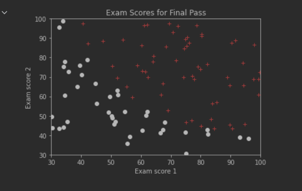
水平方向为Exam 1 Score,垂直方向为Exam 2 Score。红色+点表示Passed=1,黑色圆圈点表示Passed=0。可以观察到,所有数据点较为明显的分成两个类别(通过或不通过)。
线性回归主要都是针对训练数据和计算结果均为数值的情形。而在本例中,结果不是数值而是某种分类:考试成绩通过或不通过。在这种情况下,可以将每个类别作为一个数值结果,然后通过模型计算自变量与该分类数值结果之间的关系。逻辑回归则提供了这类问题的解决办法。
使用LogisticRegression
设置逻辑回归算法的某些属性
model = LogisticRegression(solver=‘lbfgs’)
solver–优化器:使用lbfgs算法来执行回归计算。默认使用liblinear。注意,这两种算法的结果并不相同
执行计算
model.fit(X, y)
执行预测
model.predict(newX)
返回值是newX矩阵中每行数据所对应的结果。如果是1,则表示passed;如果是0,则表示unpassed 获得模型参数值
theta0 = model.intercept_[0]
theta1 = model.coef_[0,0]
theta2 = model.coef_[0,1]
决策边界线 决策边界线可视为两种类别数据点的分界线。在该分界线的一侧,所有数据点都被归为passed类(1),另一侧的所有数据点都被归为unpassed类(0) 对于本例来说,决策边界线是一条直线(在案例2中进行了说明) theta0,theta1和theta2定义了决策边界线直线:
 其中,
其中, 表示横坐标(Exam Score 1),
 表示纵坐标(Exam Score 2),
 表示该直线的截距
''' 使用LogisticRegression进行逻辑回归 '''

import numpy as np
import matplotlib.pyplot as plt
from sklearn.linear_model import LogisticRegression

trainData = np.loadtxt(open('exam_score.csv', 'r'), delimiter=",",skiprows=1)
xTrain = trainData[:,[0,1]]          # 无需追加Intercept Item列
yTrain = trainData[:,2]

# print(trainData)
# print(xTrain)

model = LogisticRegression(solver='lbfgs')   # 使用lbfgs算法。默认是liblinear算法
model.fit(xTrain, yTrain)
newScores = np.array([[58, 67],[90, 90],[35, 38],[55, 56]])
print("预测结果:")
print(model.predict(newScores))
# 获取theta计算结果
print(model.intercept_)
print(model.coef_)
theta = np.array([model.intercept_[0], model.coef_[0,0], model.coef_[0,1]])

def initPlot():
    plt.figure()
    plt.title('Exam Scores for Final Pass')
    plt.xlabel('Exam score 1')
    plt.ylabel('Exam score 2')
    plt.axis([30, 100, 30, 100])
    return plt

plt = initPlot()
score1ForPassed = trainData[trainData[:,2] == 1, 0]
score2ForPassed = trainData[trainData[:,2] == 1, 1]
score1ForUnpassed = trainData[trainData[:,2] == 0, 0]
score2ForUnpassed = trainData[trainData[:,2] == 0, 1]
plt.plot(score1ForPassed,score2ForPassed,'r+')
plt.plot(score1ForUnpassed,score2ForUnpassed,'ko')
boundaryX = np.array([30, 50, 70, 90, 100])                 # 绘制决策边界线
boundaryY = -(theta[1] * boundaryX + theta[0]) / theta[2]   # 根据决策边界线的直线公式和x值,计算对应的y值
plt.plot(boundaryX, boundaryY, 'b-')
plt.show()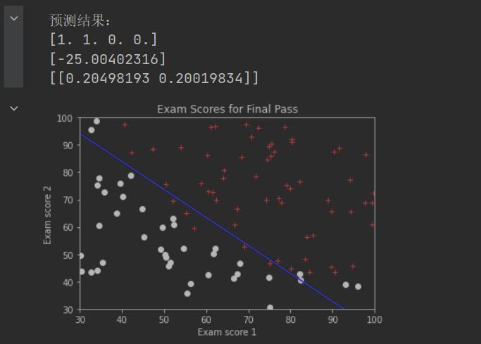
上图做出了决策边界线,该线左下方的数据点,被认为分到第0类(考试不通过),该线右上方的数据点,被认为分到第1类(考试通过)决策边界线不一定能正好把所有有本都正确的分类,除非采用更高阶的模型(而不是本例中的线性模型)。但是高阶模型也可能产生过拟合。
基于成本函数和梯度下降算法的实现
判别式/预测函数

x代表一个(行)样本数据,该样本数据共有n个变量(维度)
- 为Intercept Item,一般设置为1
g称为sigmoid激活函数,其定义为

当z=0时,g(z)的值为0.5。低于0.5的g(z)可以认为预测为false,高于0.5的预测为true。
激活函数相当于起了这样的作用:将一个连续的数值量,基于设定的阈值转变成离散的分类结果
成本函数

使用矩阵运算表达如下:

梯度计算:


计算决策边界线(Decision Boundary):
决策边界线上所有的点,其预测出来的y值 正好为0.5,即:
 当n=2时有:
  ,该边界线是一条直线
程序编写注意事项:
仔细思考成本函数和梯度计算的矩阵运算实现
先对数据进行归一化处理,有助于计算收敛
训练数据和测试数据需要手动添加Intercept Item列。先进行归一化,再手动添加Intercept Item
测试数据也需要进行相应的归一化处理,才能预测。
绘制边界线时,边界线上的点横坐标数据也需要先归一处理,然后求出归一化的纵坐标,最后再回算出纵坐标的正常值
一般情况下,测试数据、边界线数据在进行归一化处理时,都应该采用训练数据中计算出来的列平均值,而不是它们自身的平均值
''' 使用梯度下降算法进行逻辑回归 '''

%matplotlib inline
import numpy as np
import matplotlib.pyplot as plt
import bgd_resolver

def normalizeData(X, column_mean, column_std):       # 归一化
    return (X - column_mean) / column_std

def sigmoid(z):                                      #
    return 1. / (1 + np.exp(-z))

def costFn(theta, X, y):                             # 成本函数
    temp = sigmoid(X.dot(theta))
    cost = -y.dot(np.log(temp)) - (1 - y).dot(np.log(1 - temp))
    return cost / len(X)

def gradientFn(theta, X, y):                         # 梯度下降
    return xTrain.T.dot(sigmoid(xTrain.dot(theta)) - yTrain) / len(X)

def initPlot():                                      # 绘图函数
    plt.figure()
    plt.title('Exam Scores for Final Pass')
    plt.xlabel('Exam score 1')
    plt.ylabel('Exam score 2')
    plt.axis([30, 100, 30, 100])
    return plt


trainData = np.loadtxt(open('exam_score.csv', 'r'), delimiter=",",skiprows=1)
xTrain = trainData[:, [0, 1]]
# 计算训练数据每列平均值和每列的标准差
xTrain_column_mean = xTrain.mean(axis=0)
xTrain_column_std = xTrain.std(axis=0)
xTrain = normalizeData(xTrain, xTrain_column_mean, xTrain_column_std)      # 如果不进行归一化处理,计算过程中可能产生溢出(但似乎仍可以收敛)
x0 = np.ones(len(xTrain))
xTrain = np.c_[x0, xTrain]          # 需手动追加Intercept Item列
yTrain = trainData[:,2]             # 取出因变量

np.random.seed(0)
init_theta = np.random.random(3)    # 随机初始化theta
theta = bgd_resolver.batch_gradient_descent(costFn, gradientFn, init_theta, xTrain, yTrain, 0.005, 0.00001)

# 预测若干数据,也需要先归一化,使用之前训练数据的mean和std
newScores = np.array([[58, 67], [90, 90], [35, 38], [55, 56]])
newScores = normalizeData(newScores, xTrain_column_mean, xTrain_column_std)
x0 = np.ones(len(newScores))
newScores = np.c_[x0, newScores]  # 注意要添加Intercept Item
print("预测结果:")
print(sigmoid(newScores.dot(theta)))

plt = initPlot()
score1ForPassed = trainData[trainData[:,2] == 1, 0]
score2ForPassed = trainData[trainData[:,2] == 1, 1]
score1ForUnpassed = trainData[trainData[:,2] == 0, 0]
score2ForUnpassed = trainData[trainData[:,2] == 0, 1]
plt.plot(score1ForPassed,score2ForPassed,'r+')
plt.plot(score1ForUnpassed,score2ForUnpassed,'ko')

# 绘制决策边界线
boundaryX = np.array([30, 50, 70, 90, 100])
# 因为之前进行了归一化,因此边界线上点的x坐标也需要先归一化。x坐标对应的列索引是0
normalizedBoundaryX = (boundaryX - xTrain_column_mean[0]) / xTrain_column_std[0]
# 下面计算出来的边界线上的y坐标normalizedBoundaryY是经过归一化处理的坐标
normalizedBoundaryY = -(theta[1] * normalizedBoundaryX + theta[0] ) / theta[2]
# boundaryY才是将归一化坐标还原成正常坐标。y坐标对应的列索引是1
boundaryY = xTrain_column_std[1] * normalizedBoundaryY + xTrain_column_mean[1]

plt.plot(boundaryX, boundaryY, 'b-')
plt.show()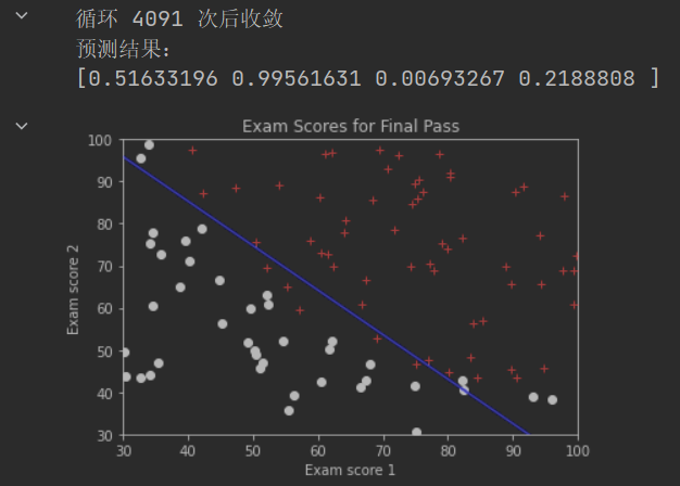
基于scipy.optimize优化运算库的实现
使用minimize库函数
需要提供jac参数,并将其设置为梯度计算函数
scipy.optimize库中提供的算法会比我们自己实现的算法更高效、灵活、全面
本例中没有对数据进行归一处理,因此导致minimize方法执行过程中溢出(尽管可能也能收敛)。请自行添加归一化处理功能
''' 使用minimize来优化逻辑回归求解 '''

%matplotlib inline
import numpy as np
import matplotlib.pyplot as plt
import scipy.optimize as opt

# 定义全局变量
trainData = np.loadtxt(open('exam_score.csv', 'r'), delimiter=",",skiprows=1)
xTrain = trainData[:,[0, 1]]
x0 = np.ones(len(xTrain))
xTrain = np.c_[x0, xTrain]
yTrain = trainData[:,2]

def sigmoid(z):
    return 1. / (1 + np.exp(-z))

# Cost Function以theta为参数
def costFn(theta, X, y):
    temp = sigmoid(xTrain.dot(theta))
    cost = -yTrain.dot(np.log(temp)) - (1 - yTrain).dot(np.log(1 - temp))
    return cost / len(X)

# Gradient Function以theta为参数
def gradientFn(theta, X, y):
    return xTrain.T.dot(sigmoid(xTrain.dot(theta)) - yTrain) / len(X)

np.random.seed(0)
# 随机初始化theta,计算过程中可能产生溢出。
# 可以尝试将init_theta乘以0.01,这样可以防止计算溢出
init_theta = np.random.random(xTrain.shape[1])
result = opt.minimize(costFn, init_theta, args=(xTrain, yTrain), method='BFGS', jac=gradientFn, options={'disp': True})
theta = result.x            # 最小化Cost时的theta

# 预测若干数据
newScores = np.array([[1, 58, 67],[1, 90,90],[1, 35,38],[1, 55,56]])  # 注意要添加Intercept Item
print("预测结果:")
print(sigmoid(newScores.dot(theta)))

def initPlot():
    plt.figure()
    plt.title('Exam Scores for Final Pass')
    plt.xlabel('Exam score 1')
    plt.ylabel('Exam score 2')
    plt.axis([30, 100, 30, 100])
    return plt

plt = initPlot()
score1ForPassed = trainData[trainData[:,2] == 1, 0]
score2ForPassed = trainData[trainData[:,2] == 1, 1]
score1ForUnpassed = trainData[trainData[:,2] == 0, 0]
score2ForUnpassed = trainData[trainData[:,2] == 0, 1]
plt.plot(score1ForPassed,score2ForPassed,'r+')
plt.plot(score1ForUnpassed,score2ForUnpassed,'ko')
boundaryX = np.array([30, 50, 70, 90, 100])                     # 绘制决策边界线
boundaryY = -(theta[1] * boundaryX + theta[0]) / theta[2]
plt.plot(boundaryX,boundaryY, 'b-')
plt.show()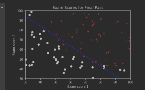


 1654
1654


 被折叠的 条评论
为什么被折叠?
被折叠的 条评论
为什么被折叠?
 到【灌水乐园】发言


