工具系列：PyCaret介绍_多分类代码示例

数智笔记

已于 2023-12-20 13:41:12 修改

阅读量1.6k

点赞数 23

分类专栏： PyCaret 数据挖掘文章标签：分类数据挖掘人工智能

于 2023-12-19 13:22:02 首次发布

本文链接：https://blog.csdn.net/wjjc1017/article/details/135081861

版权

数据挖掘同时被 2 个专栏收录

163 篇文章 11 订阅

订阅专栏

PyCaret

14 篇文章 1 订阅

订阅专栏

👋 工具系列：PyCaret介绍_多分类代码示例

PyCaret 介绍

PyCaret是一个开源的、低代码的Python机器学习库，可以自动化机器学习工作流程。它是一个端到端的机器学习和模型管理工具，可以大大加快实验周期并提高生产效率。

与其他开源机器学习库相比，PyCaret是一个替代低代码库，可以用几行代码代替数百行代码。这使得实验速度指数级增加，效率更高。PyCaret本质上是围绕几个机器学习库和框架（如scikit-learn、XGBoost、LightGBM、CatBoost、spaCy、Optuna、Hyperopt、Ray等）的Python封装。

PyCaret的设计和简洁性受到了Gartner首次使用的公民数据科学家这一新兴角色的启发。公民数据科学家是能够执行简单和中等复杂的分析
任务的高级用户，而以前这些任务需要更多的技术专长。

# 导入pycaret库
import pycaret

# 打印pycaret库的版本号
pycaret.__version__

'3.0.0'

🚀 快速开始

PyCaret的分类模块是一个监督式机器学习模块，用于将元素分类到不同的组中。其目标是预测离散且无序的分类标签。

一些常见的用例包括预测客户是否违约（是或否）、预测客户流失（客户会离开还是留下）以及发现的疾病（阳性或阴性）。

该模块可用于二分类或多分类问题。它提供了几种预处理功能，通过设置函数来准备建模数据。它拥有超过18种可直接使用的算法和多个绘图功能，用于分析训练模型的性能。

在PyCaret中，典型的工作流程按照以下5个步骤顺序进行：

设置 ➡️ 比较模型 ➡️ 分析模型 ➡️ 预测 ➡️ 保存模型

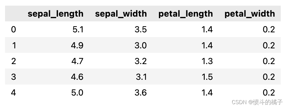
# 从pycaret数据集模块加载示例数据集
from pycaret.datasets import get_data
data = get_data('iris')

请添加图片描述

设置

此函数初始化训练环境并创建转换流水线。在执行PyCaret中的任何其他函数之前，必须调用设置函数。它只有两个必需的参数，即data和target。所有其他参数都是可选的。

# 导入pycaret分类模块和初始化设置
from pycaret.classification import *

# 初始化设置
# data: 数据集，包含特征和目标变量
# target: 目标变量的名称
# session_id: 用于重现实验结果的随机种子
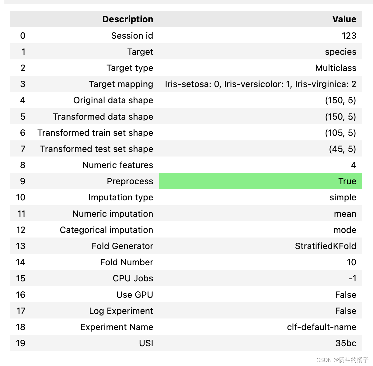
s = setup(data, target='species', session_id=123)

请添加图片描述

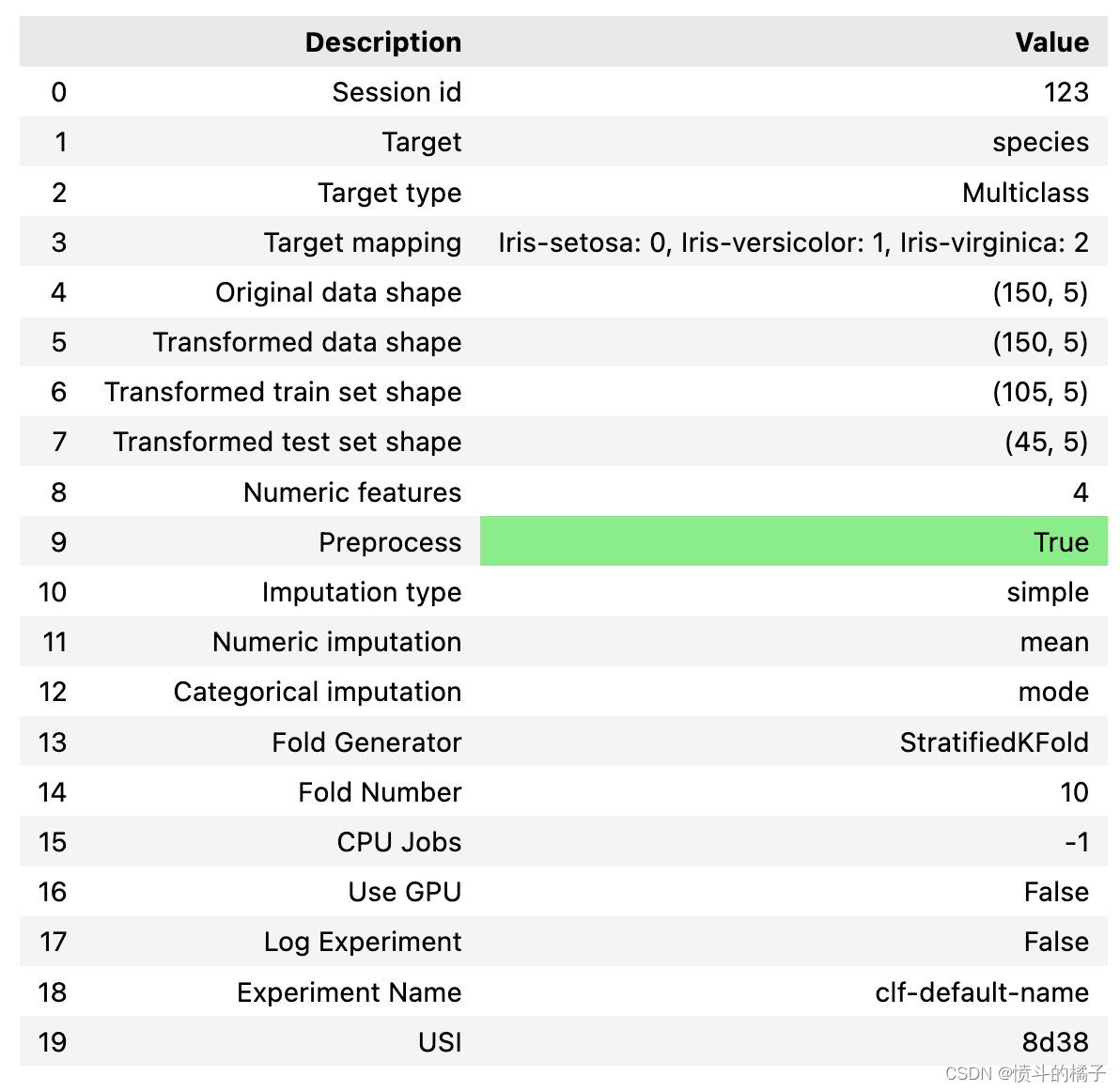
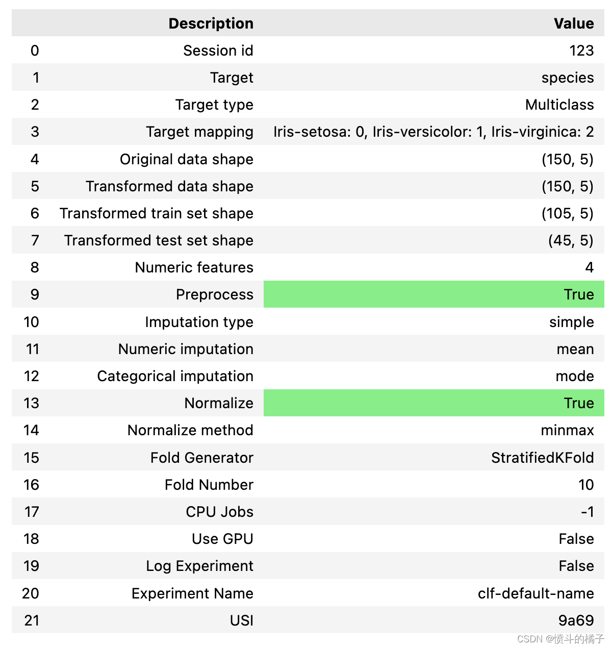
一旦设置成功执行，它将显示包含实验级别信息的信息网格。

会话ID： 一个伪随机数，在所有函数中分布为种子，以便以后可以重现。如果没有传递session_id，则会自动生成一个随机数，并分发给所有函数。
目标类型： 二进制、多类别或回归。目标类型会自动检测。
标签编码： 当目标变量为字符串类型（例如’Yes’或’No’）而不是1或0时，它会自动将标签编码为1和0，并显示映射关系（0：No，1：Yes）供参考。在本教程中，不需要进行标签编码，因为目标变量是数值类型。
原始数据形状： 在进行任何转换之前的原始数据形状。
转换后的训练集形状： 转换后的训练集形状。
转换后的测试集形状： 转换后的测试集形状。
数值特征： 被视为数值的特征数量。
分类特征： 被视为分类的特征数量。

PyCaret的API

PyCaret有两套可以使用的API。 (1) 函数式API（如上所示）和 (2) 面向对象的API。

使用面向对象的API时，您将导入一个类并执行该类的方法，而不是直接执行函数。

# 导入ClassificationExperiment类并初始化该类
from pycaret.classification import ClassificationExperiment
exp = ClassificationExperiment()

# 检查exp的类型

pycaret.classification.oop.ClassificationExperiment

# 初始化实验设置
exp.setup(data, target='species', session_id=123) 
# data: 数据集，用于训练和测试模型
# target: 目标变量，即要预测的变量
# session_id: 实验的会话ID，用于复现实验结果

请添加图片描述

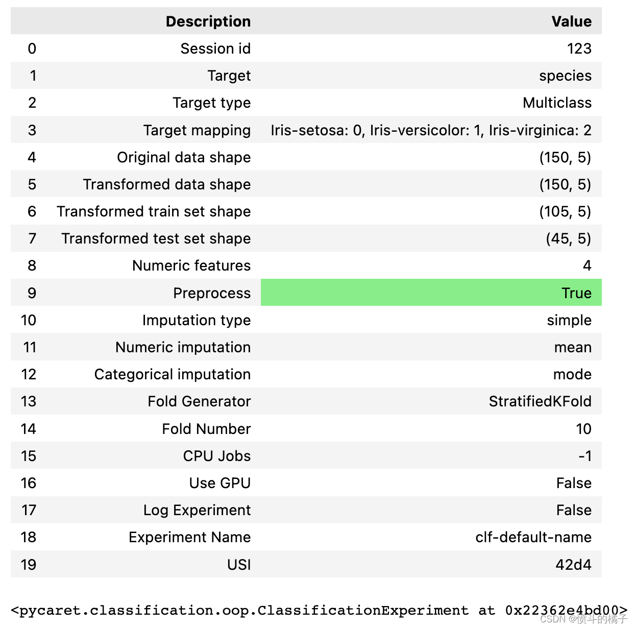
<pycaret.classification.oop.ClassificationExperiment at 0x22362e4bd00>

你可以使用任何一种方法，即函数式或面向对象编程，并且可以在两组API之间来回切换。方法的选择不会影响结果，并且已经进行了一致性测试。

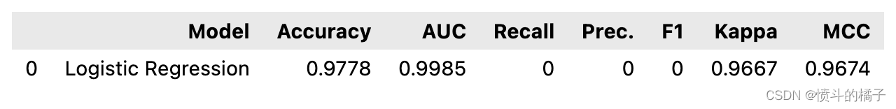
比较模型

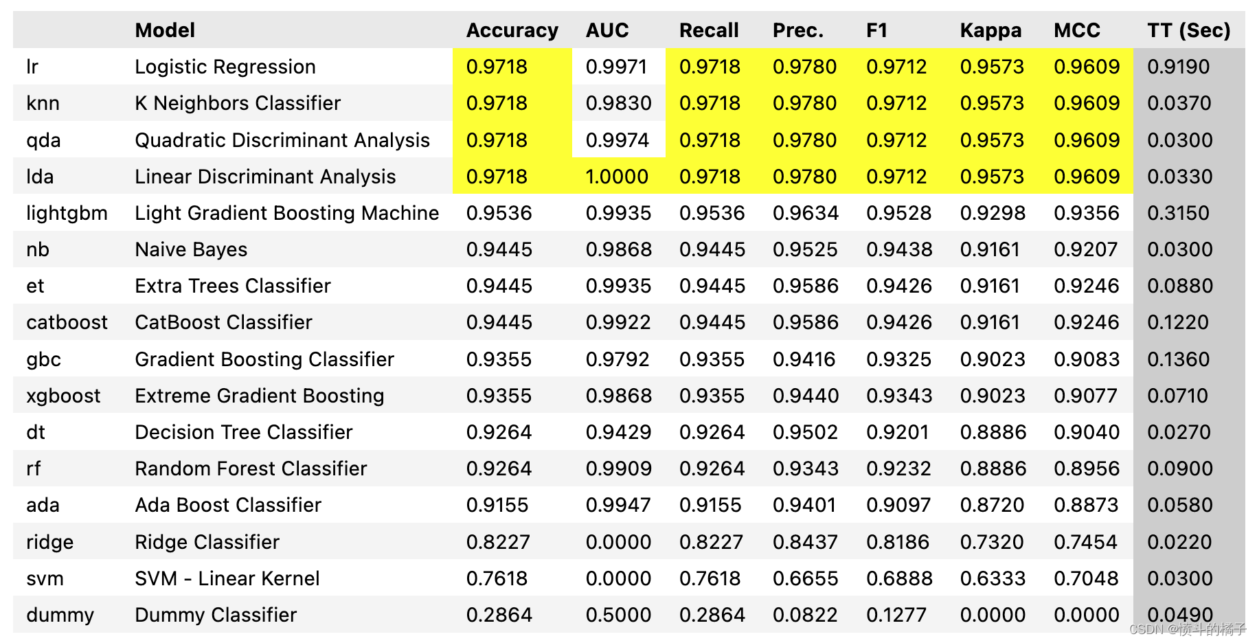
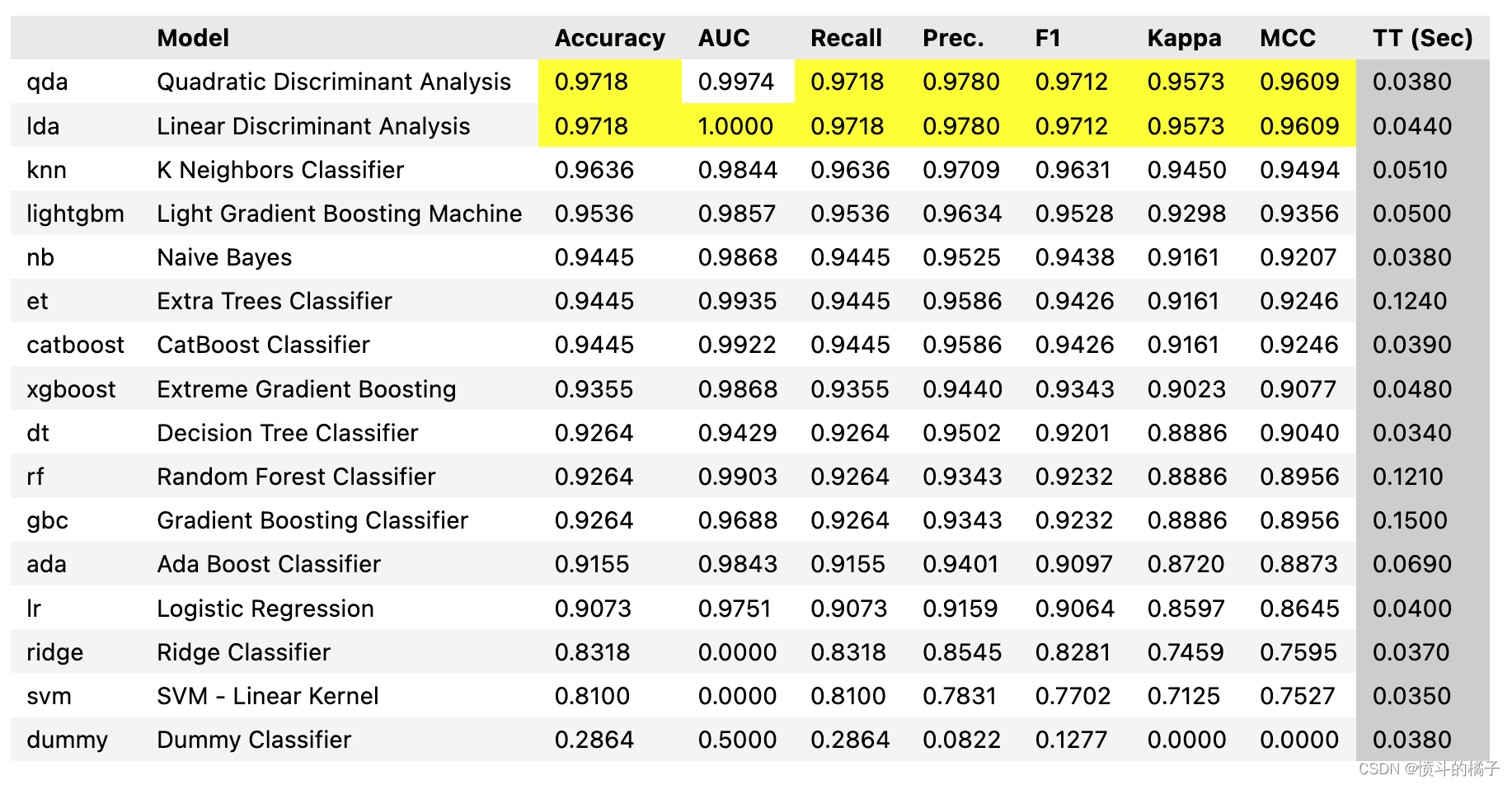
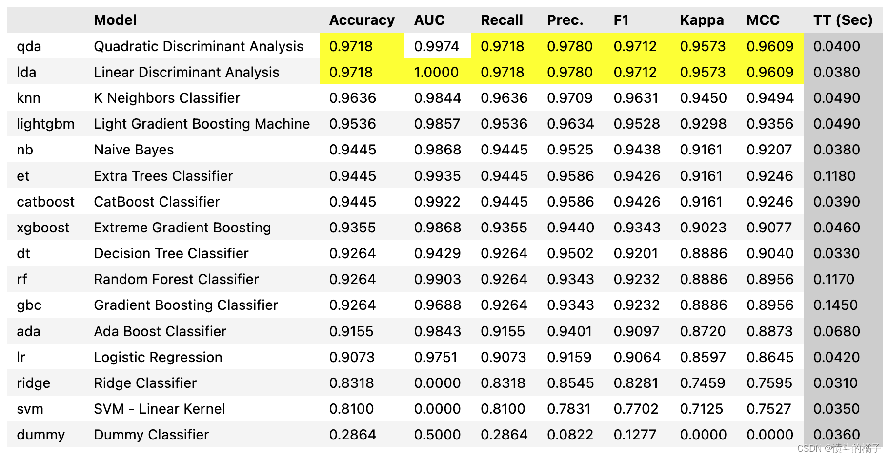
该函数使用交叉验证训练和评估模型库中所有可用的估计器的性能。该函数的输出是一个带有平均交叉验证分数的评分表。可以使用get_metrics函数访问CV期间评估的指标。可以使用add_metric和remove_metric函数添加或删除自定义指标。

# 比较基准模型

# 使用compare_models()函数比较不同的基准模型，并返回最佳模型

best = compare_models()

在这里插入图片描述

Processing:   0%|          | 0/69 [00:00<?, ?it/s]

# 比较模型
exp.compare_models()

在这里插入图片描述

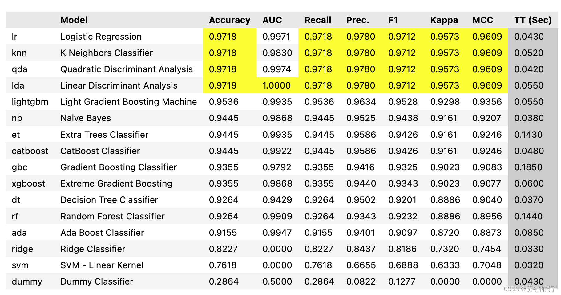
Processing:   0%|          | 0/69 [00:00<?, ?it/s]

请添加图片描述

注意，函数式API和面向对象API之间的输出是一致的。本笔记本中的其余函数将只使用函数式API显示。

分析模型

您可以使用plot_model函数来分析训练模型在测试集上的性能。在某些情况下，可能需要重新训练模型。

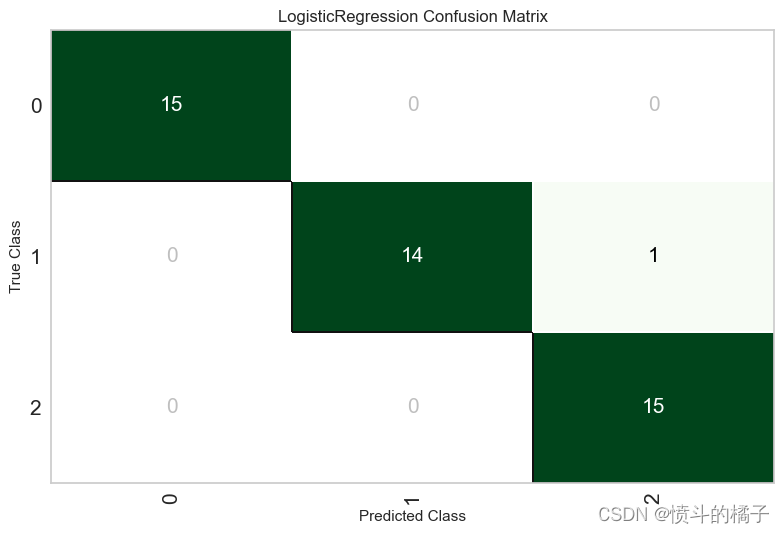
# 调用函数绘制混淆矩阵
plot_confusion_matrix(best)

在这里插入图片描述

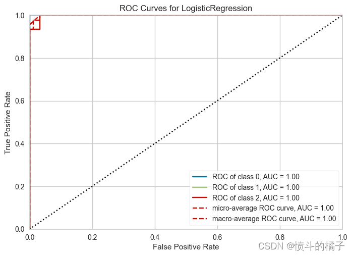
# 绘制AUC曲线
# 参数best是训练好的模型
# 参数plot='auc'表示绘制AUC曲线
plot_model(best, plot='auc')

在这里插入图片描述

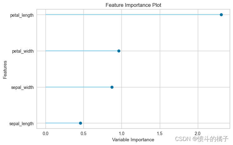
# 绘制特征重要性图
# best是训练好的模型
# plot参数设置为'feature'，表示绘制特征重要性图
plot_model(best, plot='feature')

在这里插入图片描述


# 使用help函数查看plot_model函数的文档字符串，以了解可用的绘图选项
help(plot_model)

Help on function plot_model in module pycaret.classification.functional:

plot_model(estimator, plot: str = 'auc', scale: float = 1, save: bool = False, fold: Union[int, Any, NoneType] = None, fit_kwargs: Union[dict, NoneType] = None, plot_kwargs: Union[dict, NoneType] = None, groups: Union[str, Any, NoneType] = None, verbose: bool = True, display_format: Union[str, NoneType] = None) -> Union[str, NoneType]
    This function analyzes the performance of a trained model on holdout set.
    It may require re-training the model in certain cases.
    
    Example
    -------
    >>> from pycaret.datasets import get_data
    >>> juice = get_data('juice')
    >>> from pycaret.classification import *
    >>> exp_name = setup(data = juice,  target = 'Purchase')
    >>> lr = create_model('lr')
    >>> plot_model(lr, plot = 'auc')
    
    
    estimator: scikit-learn compatible object
        Trained model object
    
    
    plot: str, default = 'auc'
        List of available plots (ID - Name):
    
        * 'pipeline' - Schematic drawing of the preprocessing pipeline
        * 'auc' - Area Under the Curve
        * 'threshold' - Discrimination Threshold
        * 'pr' - Precision Recall Curve
        * 'confusion_matrix' - Confusion Matrix
        * 'error' - Class Prediction Error
        * 'class_report' - Classification Report
        * 'boundary' - Decision Boundary
        * 'rfe' - Recursive Feature Selection
        * 'learning' - Learning Curve
        * 'manifold' - Manifold Learning
        * 'calibration' - Calibration Curve
        * 'vc' - Validation Curve
        * 'dimension' - Dimension Learning
        * 'feature' - Feature Importance
        * 'feature_all' - Feature Importance (All)
        * 'parameter' - Model Hyperparameter
        * 'lift' - Lift Curve
        * 'gain' - Gain Chart
        * 'tree' - Decision Tree
        * 'ks' - KS Statistic Plot
    
    
    scale: float, default = 1
        The resolution scale of the figure.
    
    
    save: bool, default = False
        When set to True, plot is saved in the current working directory.
    
    
    fold: int or scikit-learn compatible CV generator, default = None
        Controls cross-validation. If None, the CV generator in the ``fold_strategy``
        parameter of the ``setup`` function is used. When an integer is passed,
        it is interpreted as the 'n_splits' parameter of the CV generator in the
        ``setup`` function.
    
    
    fit_kwargs: dict, default = {} (empty dict)
        Dictionary of arguments passed to the fit method of the model.
    
    
    plot_kwargs: dict, default = {} (empty dict)
        Dictionary of arguments passed to the visualizer class.
            - pipeline: fontsize -> int
    
    
    groups: str or array-like, with shape (n_samples,), default = None
        Optional group labels when GroupKFold is used for the cross validation.
        It takes an array with shape (n_samples, ) where n_samples is the number
        of rows in training dataset. When string is passed, it is interpreted as
        the column name in the dataset containing group labels.
    
    
    verbose: bool, default = True
        When set to False, progress bar is not displayed.
    
    
    display_format: str, default = None
        To display plots in Streamlit (https://www.streamlit.io/), set this to 'streamlit'.
        Currently, not all plots are supported.
    
    
    Returns:
        Path to saved file, if any.
    
    
    Warnings
    --------
    -   Estimators that does not support 'predict_proba' attribute cannot be used for
        'AUC' and 'calibration' plots.
    
    -   When the target is multiclass, 'calibration', 'threshold', 'manifold' and 'rfe'
        plots are not available.
    
    -   When the 'max_features' parameter of a trained model object is not equal to
        the number of samples in training set, the 'rfe' plot is not available.

一种替代plot_model函数的方法是evaluate_model。它只能在Notebook中使用，因为它使用了ipywidget。

evaluate_model(best)

interactive(children=(ToggleButtons(description='Plot Type:', icons=('',), options=(('Pipeline Plot', 'pipelin…

预测

predict_model 函数会在数据框中返回 prediction_label 和 prediction_score（预测类别的概率）作为新的列。当数据为 None（默认值）时，它会使用在设置函数期间创建的测试集进行评分。

# 预测测试集数据
# 使用之前训练好的模型对测试集数据进行预测
holdout_pred = predict_model(best)

在这里插入图片描述

# 展示预测结果的数据框

# 使用head()函数显示数据框的前几行，默认显示前5行

holdout_pred.head()

在这里插入图片描述

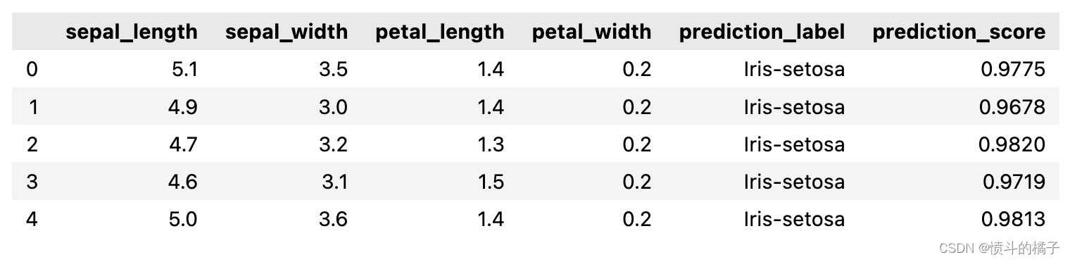
相同的函数可以用于预测未见数据集上的标签。让我们创建原始数据的副本并删除“Class变量”。然后，我们可以使用没有标签的新数据框进行评分。

# 复制数据并删除Class变量

# 复制原始数据到新的数据集new_data
new_data = data.copy()

# 在新数据集new_data中删除'species'列，axis=1表示按列删除
new_data.drop('species', axis=1, inplace=True)

# 显示新数据集new_data的前几行数据
new_data.head()

在这里插入图片描述


# 使用预训练的模型对新数据进行预测
predictions = predict_model(best, data=new_data)

# 显示预测结果的前几行
predictions.head()

在这里插入图片描述

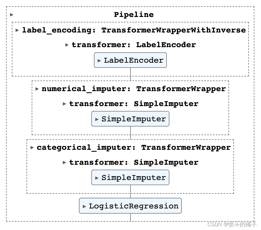
保存模型

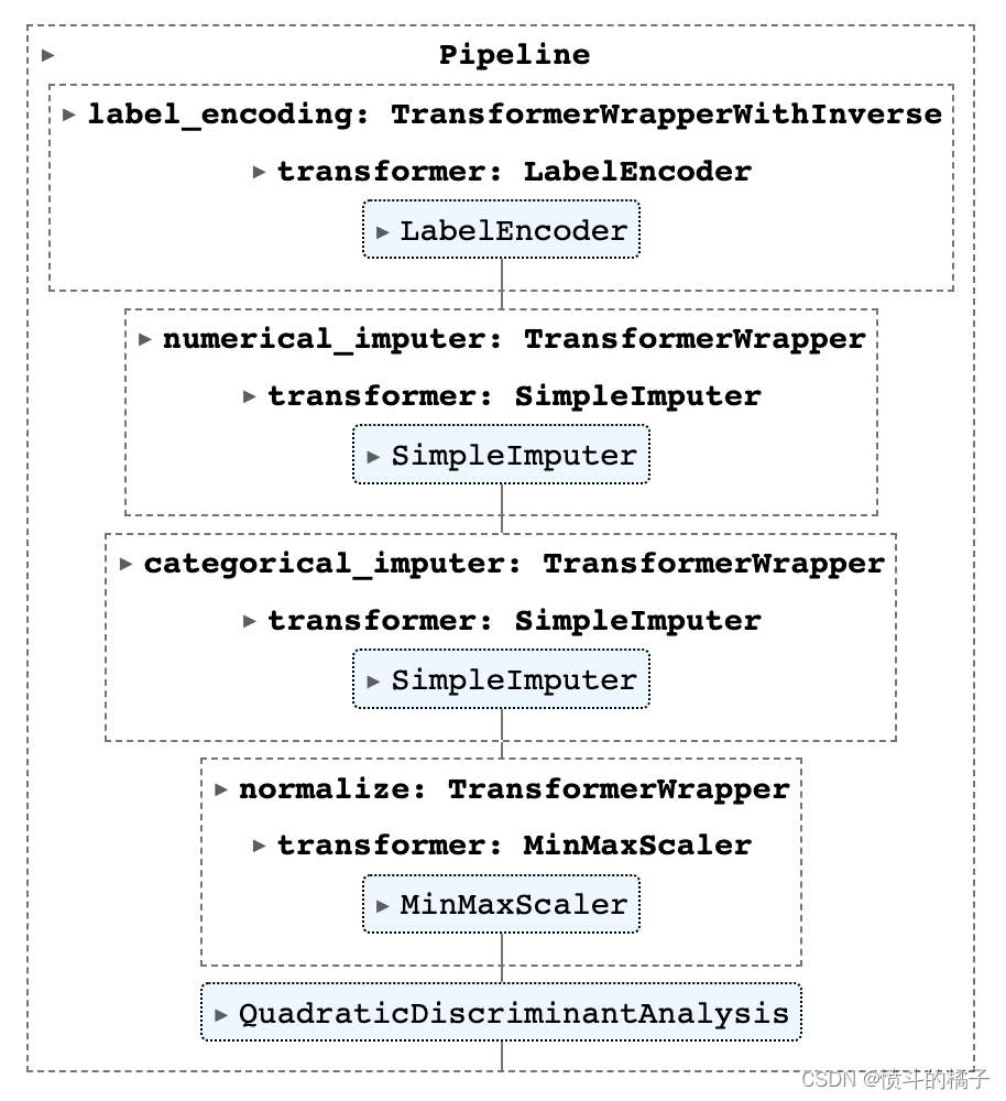
最后，您可以使用pycaret的save_model函数将整个流水线保存到磁盘上以供以后使用。

# 调用save_model函数，将最佳模型保存为名为'my_first_pipeline'的文件
save_model(best, 'my_first_pipeline')

Transformation Pipeline and Model Successfully Saved





(Pipeline(memory=FastMemory(location=C:\Users\owner\AppData\Local\Temp\joblib),
          steps=[('label_encoding',
                  TransformerWrapperWithInverse(exclude=None, include=None,
                                                transformer=LabelEncoder())),
                 ('numerical_imputer',
                  TransformerWrapper(exclude=None,
                                     include=['sepal_length', 'sepal_width',
                                              'petal_length', 'petal_width'],
                                     transformer=SimpleImputer(add_indicator=F...
                                                               fill_value=None,
                                                               missing_values=nan,
                                                               strategy='most_frequent',
                                                               verbose='deprecated'))),
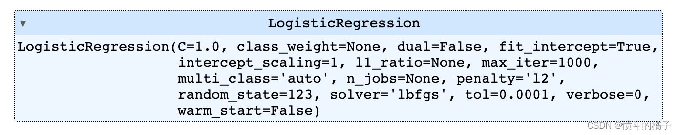
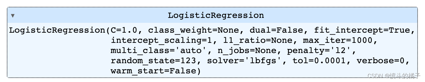
                 ('trained_model',
                  LogisticRegression(C=1.0, class_weight=None, dual=False,
                                     fit_intercept=True, intercept_scaling=1,
                                     l1_ratio=None, max_iter=1000,
                                     multi_class='auto', n_jobs=None,
                                     penalty='l2', random_state=123,
                                     solver='lbfgs', tol=0.0001, verbose=0,
                                     warm_start=False))],
          verbose=False),
 'my_first_pipeline.pkl')

# 加载模型
loaded_best_pipeline = load_model('my_first_pipeline')

# 加载已经训练好的最佳模型

# 返回已加载的最佳模型的结果

Transformation Pipeline and Model Successfully Loaded

请添加图片描述

👇 详细的函数功能概述

✅ 设置

这个函数在PyCaret中初始化实验，并根据传入函数的所有参数创建转换流水线。在执行任何其他函数之前，必须调用设置函数。它接受两个必需参数：data和target。所有其他参数都是可选的，并用于配置数据预处理流水线。


# 设置数据集和目标变量
# data: 数据集
# target: 目标变量，即要预测的变量
# session_id: 用于重现实验结果的随机种子
s = setup(data, target='species', session_id=123)

在这里插入图片描述

要访问由设置函数创建的所有变量，例如转换后的数据集、随机状态等，您可以使用get_config方法。

# 获取所有可用的配置信息
get_config()

{'USI',
 'X',
 'X_test',
 'X_test_transformed',
 'X_train',
 'X_train_transformed',
 'X_transformed',
 '_available_plots',
 '_ml_usecase',
 'data',
 'dataset',
 'dataset_transformed',
 'exp_id',
 'exp_name_log',
 'fix_imbalance',
 'fold_generator',
 'fold_groups_param',
 'fold_shuffle_param',
 'gpu_n_jobs_param',
 'gpu_param',
 'html_param',
 'idx',
 'is_multiclass',
 'log_plots_param',
 'logging_param',
 'memory',
 'n_jobs_param',
 'pipeline',
 'seed',
 'target_param',
 'test',
 'test_transformed',
 'train',
 'train_transformed',
 'variable_and_property_keys',
 'variables',
 'y',
 'y_test',
 'y_test_transformed',
 'y_train',
 'y_train_transformed',
 'y_transformed'}

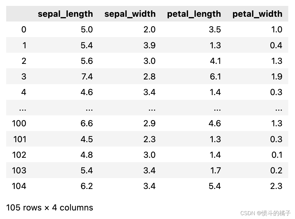
# 获取X_train_transformed的配置信息
get_config('X_train_transformed')

在这里插入图片描述

# 打印当前的种子值
print("当前的种子值为: {}".format(get_config('seed')))

# 使用set_config函数来改变种子值
set_config('seed', 786)
print("新的种子值为: {}".format(get_config('seed')))

The current seed is: 123
The new seed is: 786

所有的预处理配置和实验设置/参数都传递给setup函数。要查看所有可用的参数，请检查docstring：

# help(setup)

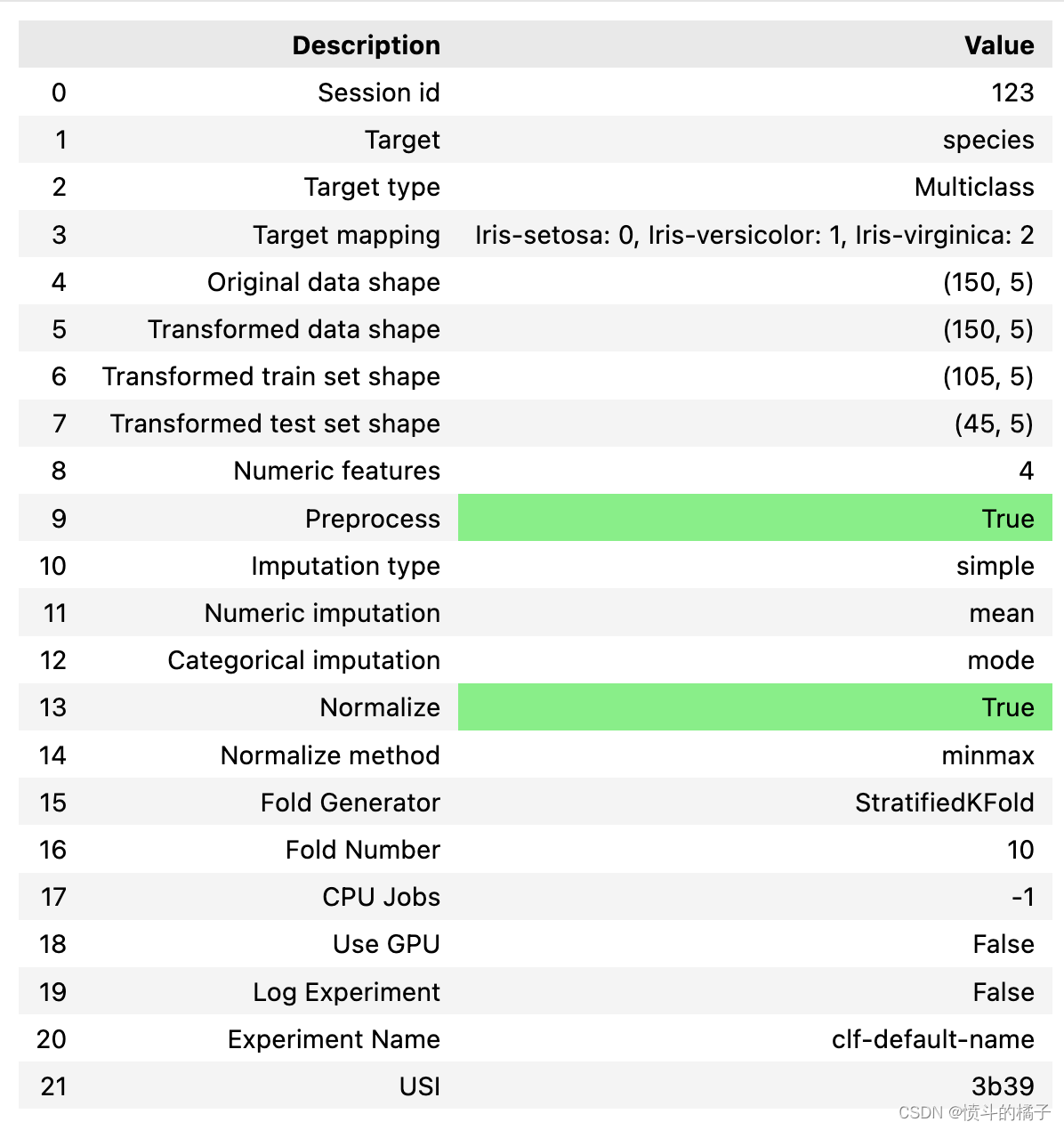
# 初始化设置，设置normalize为True
# 参数data为数据集，target为目标变量的名称，session_id为随机种子，normalize为是否对数据进行归一化处理，normalize_method为归一化方法
s = setup(data, target='species', session_id=123, normalize=True, normalize_method='minmax')

在这里插入图片描述

# 获取X_train_transformed的配置信息，并查看'sepal_length'列的直方图

# 使用get_config函数获取X_train_transformed的配置信息
config = get_config('X_train_transformed')

# 获取'sepal_length'列，并绘制直方图
config['sepal_length'].hist()

<AxesSubplot:>

在这里插入图片描述

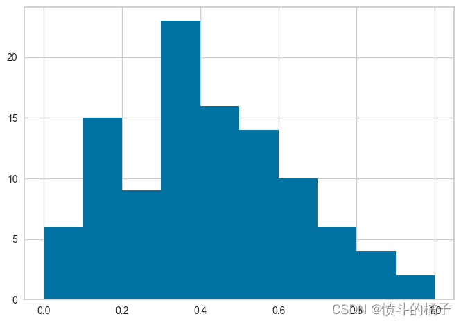
请注意，所有的值都在0和1之间 - 这是因为我们在setup函数中传递了normalize=True。如果你不记得它与实际数据的比较方式，没问题 - 我们也可以使用get_config来访问非转换的值，然后进行比较。请参见下面的内容，并注意x轴上的值范围，并将其与上面的直方图进行比较。

# 获取配置文件中的X_train数据集，并选择其中的'sepal_length'列
X_train = get_config('X_train')['sepal_length']

# 绘制'sepal_length'列的直方图
X_train.hist()

<AxesSubplot:>

在这里插入图片描述

✅ 比较模型

该函数使用交叉验证训练和评估模型库中所有可用的估计器的性能。该函数的输出是一个带有平均交叉验证分数的评分网格。可以使用get_metrics函数访问CV期间评估的指标。可以使用add_metric和remove_metric函数添加或删除自定义指标。

# 比较模型函数，用于选择最佳模型
best = compare_models()

在这里插入图片描述

Processing:   0%|          | 0/69 [00:00<?, ?it/s]

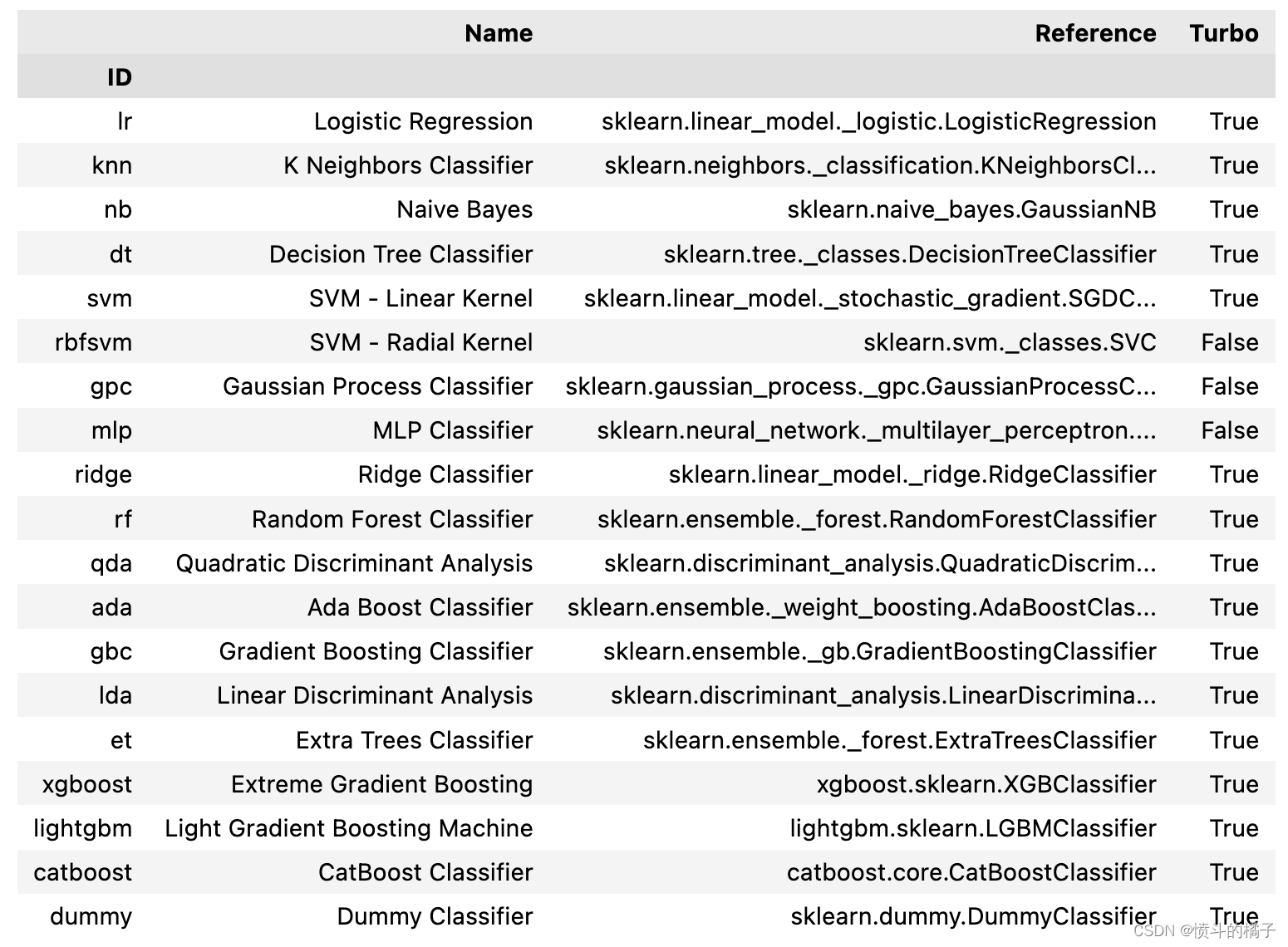
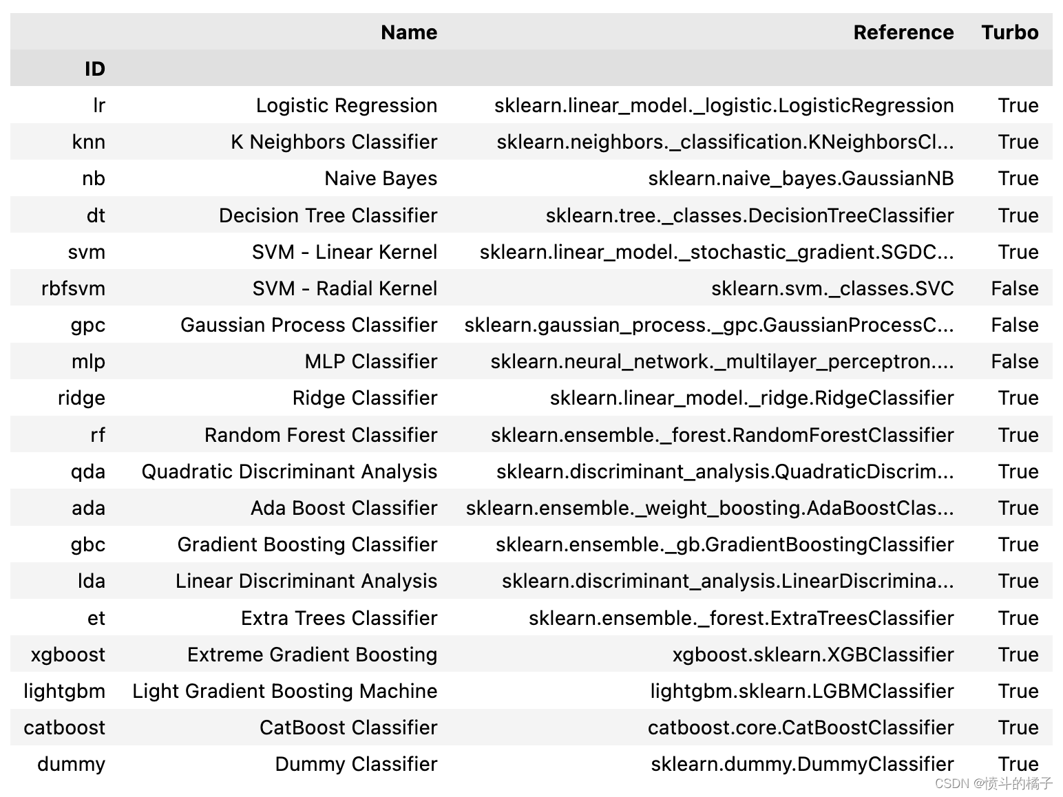
compare_models 默认使用模型库中的所有估计器（除了 Turbo=False 的模型）。要查看所有可用的模型，您可以使用函数 models()。

# 使用transformers库中的models()函数来获取可用的模型列表
available_models = models()

# 打印可用的模型列表
print(available_models)

在这里插入图片描述

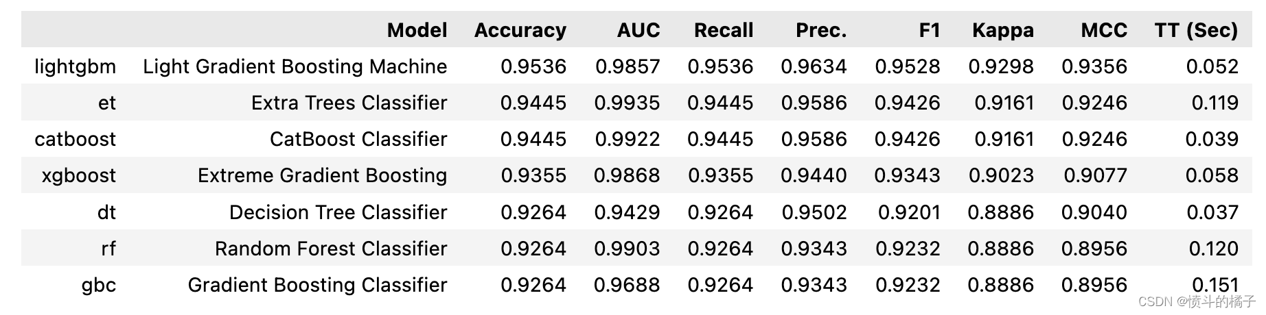
你可以在compare_models中使用include和exclude参数，只训练选择的模型或通过在exclude参数中传递模型id来排除特定的模型。

# 使用compare_models函数比较不同的决策树模型
# include参数指定了要比较的模型，包括决策树（dt）、随机森林（rf）、极端随机树（et）、梯度提升树（gbc）、XGBoost（xgboost）、LightGBM（lightgbm）和CatBoost（catboost）
compare_tree_models = compare_models(include=['dt', 'rf', 'et', 'gbc', 'xgboost', 'lightgbm', 'catboost'])

在这里插入图片描述

Processing:   0%|          | 0/33 [00:00<?, ?it/s]

compare_tree_models

请添加图片描述

功能上面的函数返回训练好的模型对象作为输出。评分网格只显示，不返回。如果您需要访问评分网格，可以使用pull函数访问数据框。

# 从数据源中获取比较树模型结果的数据

compare_tree_models_results = pull()

在这里插入图片描述

默认情况下，compare_models函数返回基于sort参数中定义的指标的最佳性能模型。让我们修改我们的代码，返回基于Recall的前3个最佳模型。

# 使用compare_models函数来比较不同模型的性能
# sort参数设置为'Recall'，表示按照召回率对模型进行排序
# n_select参数设置为3，表示选择召回率最高的3个模型
best_recall_models_top3 = compare_models(sort='Recall', n_select=3)

在这里插入图片描述

Processing:   0%|          | 0/71 [00:00<?, ?it/s]

# 定义一个列表，用于存储前三个Recall最高的模型的名称
best_recall_models_top3

[QuadraticDiscriminantAnalysis(priors=None, reg_param=0.0,
                               store_covariance=False, tol=0.0001),
 LinearDiscriminantAnalysis(covariance_estimator=None, n_components=None,
                            priors=None, shrinkage=None, solver='svd',
                            store_covariance=False, tol=0.0001),
 KNeighborsClassifier(algorithm='auto', leaf_size=30, metric='minkowski',
                      metric_params=None, n_jobs=-1, n_neighbors=5, p=2,
                      weights='uniform')]

一些在compare_models中可能非常有用的其他参数包括：

fold
cross_validation
budget_time
errors
probability_threshold
parallel

您可以查看函数的文档字符串以获取更多信息。

# help(compare_models)

✅ 实验日志记录

PyCaret与许多不同类型的实验记录器集成（默认为’mlflow’）。要在PyCaret中启用实验跟踪，您可以设置log_experiment和experiment_name参数。它将根据定义的记录器自动跟踪所有指标、超参数和工件。



# 设置实验
# data: 数据集
# target: 目标变量
# log_experiment: 是否记录实验日志到mlflow
# experiment_name: 实验名称
s = setup(data, target='Class variable', log_experiment='mlflow', experiment_name='iris_experiment')

# 比较模型

# 使用compare_models()函数来比较不同的模型，找出最佳的模型

best = compare_models()

# start mlflow server on localhost:5000
# !mlflow ui

默认情况下，PyCaret使用MLFlow记录器，可以使用log_experiment参数进行更改。以下记录器可用：

mlflow
wandb
comet_ml
dagshub

您可能会发现有用的其他与日志记录相关的参数有：

experiment_custom_tags
log_plots
log_data
log_profile

有关更多信息，请查看setup函数的文档字符串。

# help(setup)

✅ 创建模型

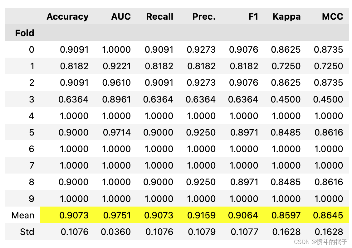
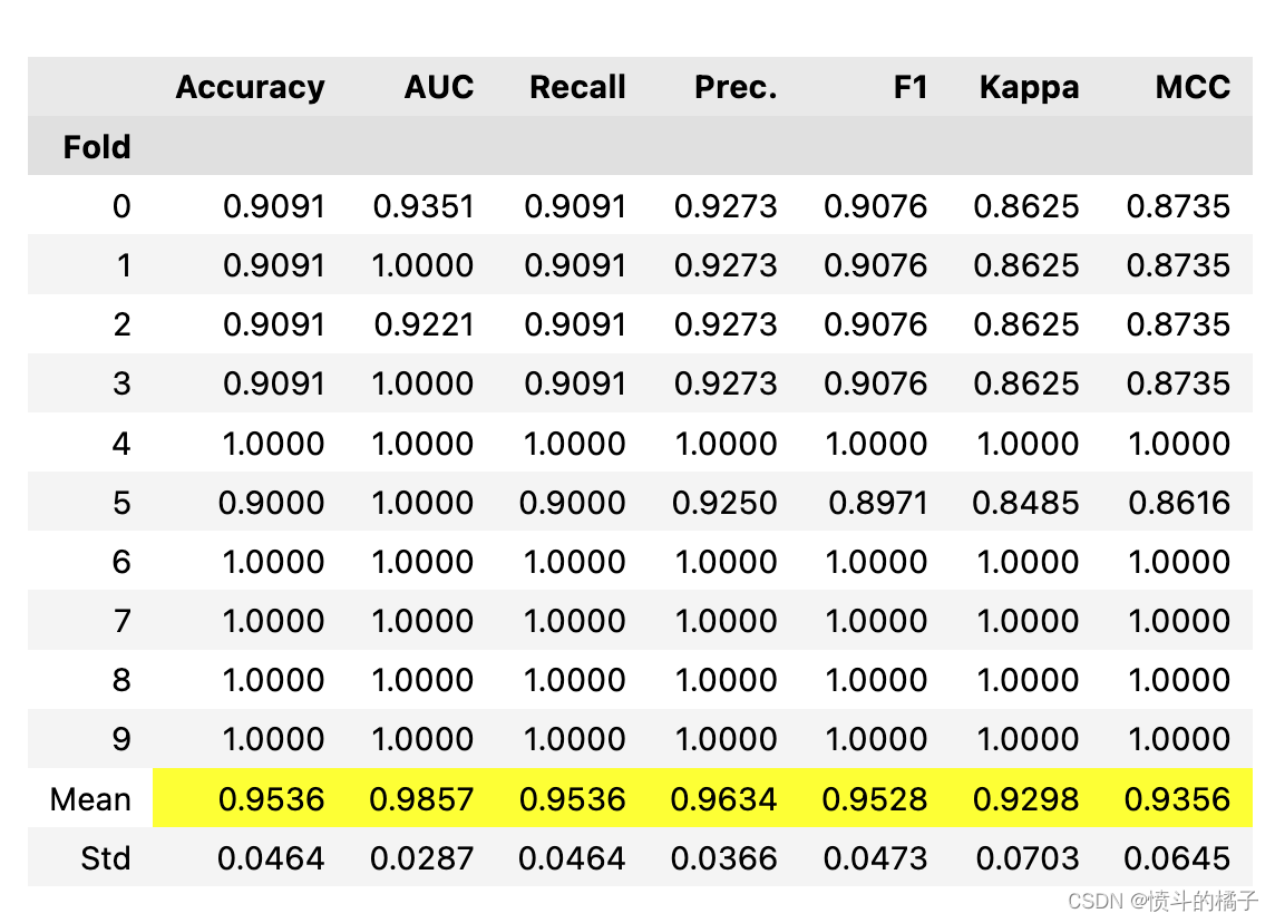
该函数使用交叉验证训练和评估给定估计器的性能。该函数的输出是一个包含每个折叠的CV分数的评分网格。可以使用get_metrics函数访问CV期间评估的指标。可以使用add_metric和remove_metric函数添加或删除自定义指标。可以使用models函数访问所有可用的模型。

# 查看所有可用的模型
models()

在这里插入图片描述

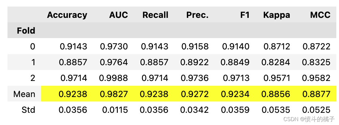
# 使用默认的折叠数（fold=10）训练逻辑回归模型
lr = create_model('lr')

在这里插入图片描述

Processing:   0%|          | 0/4 [00:00<?, ?it/s]

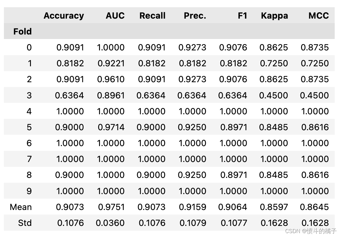
功能以上返回训练好的模型对象作为输出。评分表格仅显示而不返回。如果您需要访问评分表格，可以使用pull函数来访问数据框。

# 从pull()函数中获取lr_results变量的值
lr_results = pull()

# 打印lr_results的数据类型
print(type(lr_results))

# 打印lr_results的值
print(lr_results)

<class 'pandas.core.frame.DataFrame'>

在这里插入图片描述

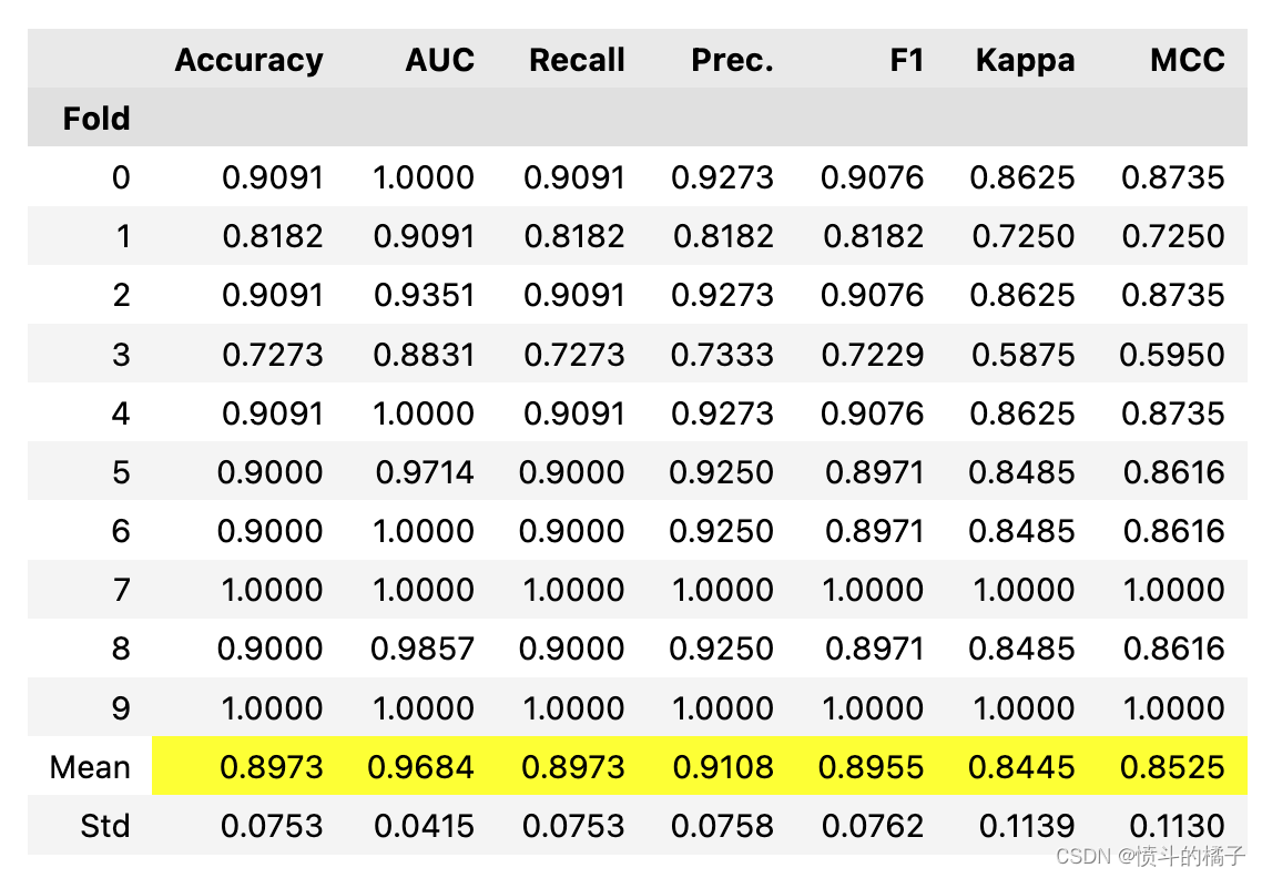
# 创建一个逻辑回归模型，并设置交叉验证的折数为3
lr = create_model('lr', fold=3)

在这里插入图片描述

Processing:   0%|          | 0/4 [00:00<?, ?it/s]

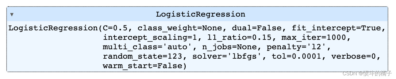
# 定义一个函数create_model，用于训练逻辑回归模型，并设置特定的模型参数
# 参数说明：
# - model_type: 模型类型，这里为逻辑回归模型，使用缩写'lr'表示
# - C: 正则化强度的倒数，用于控制模型的复杂度，数值越小表示正则化强度越大，默认为0.5
# - l1_ratio: L1正则化的比例，用于控制L1正则化的强度，数值越大表示L1正则化的强度越大，默认为0.15
create_model(model_type, C=0.5, l1_ratio=0.15):

在这里插入图片描述

Processing:   0%|          | 0/4 [00:00<?, ?it/s]

请添加图片描述

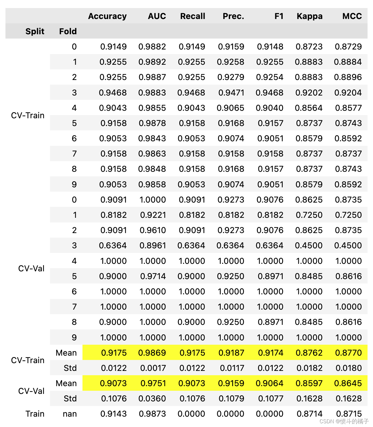
# 定义一个函数create_model，用于训练逻辑回归模型，并返回训练得分和交叉验证得分
create_model('lr', return_train_score=True)

在这里插入图片描述

Processing:   0%|          | 0/4 [00:00<?, ?it/s]

请添加图片描述

一些在create_model中可能非常有用的其他参数有：

cross_validation
engine
fit_kwargs
groups

您可以查看函数的文档字符串以获取更多信息。

# help(create_model)

✅ 调整模型

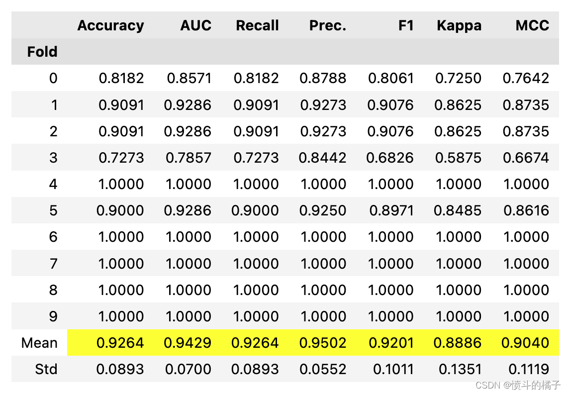
该函数用于调整模型的超参数。该函数的输出是一个通过交叉验证得到的得分网格。根据 optimize 参数中定义的指标选择最佳模型。可以使用 get_metrics 函数访问在交叉验证期间评估的指标。可以使用 add_metric 和 remove_metric 函数添加或删除自定义指标。


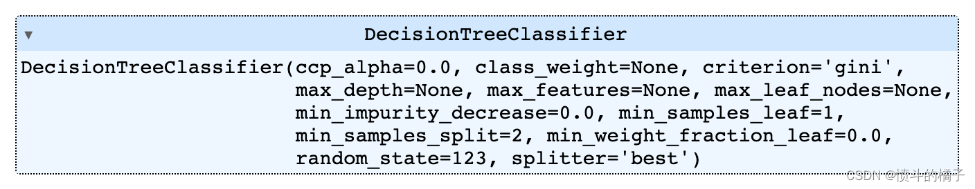
# 使用默认参数创建一个决策树模型
dt = create_model('dt')

在这里插入图片描述

Processing:   0%|          | 0/4 [00:00<?, ?it/s]

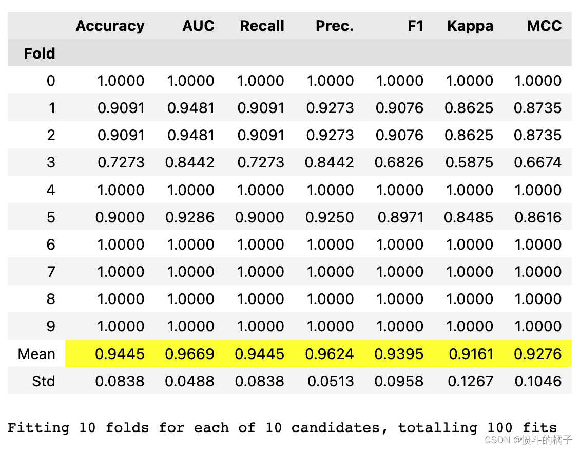
# 调整决策树模型的超参数

# 使用tune_model函数对决策树模型进行超参数调整，并将调整后的模型保存在tuned_dt变量中。
tuned_dt = tune_model(dt)

在这里插入图片描述

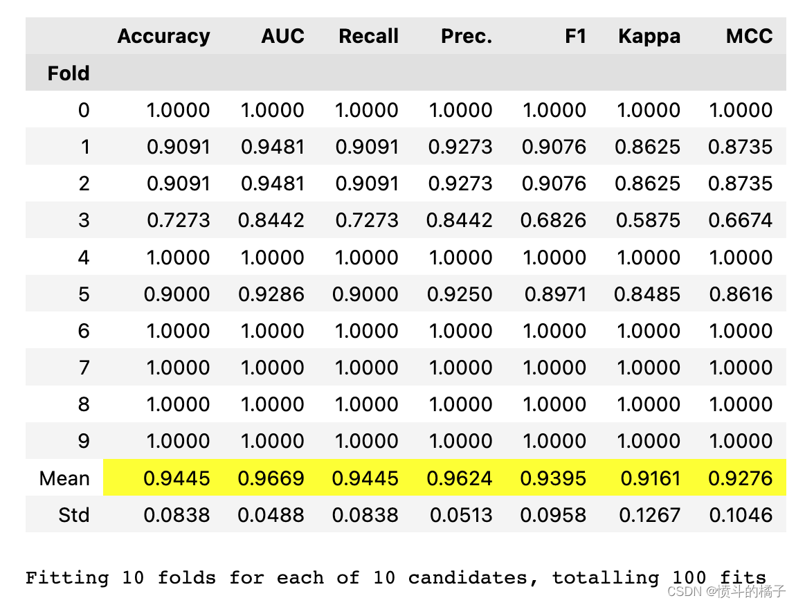
Processing:   0%|          | 0/7 [00:00<?, ?it/s]


Fitting 10 folds for each of 10 candidates, totalling 100 fits

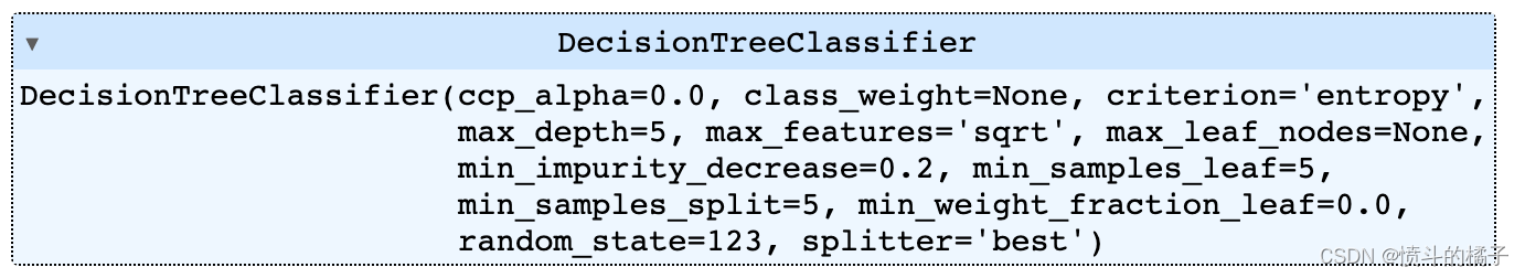
可以在optimize参数中定义要优化的度量标准（默认为’Accuracy’）。此外，还可以通过custom_grid参数传递自定义调整的网格。

dt

请添加图片描述

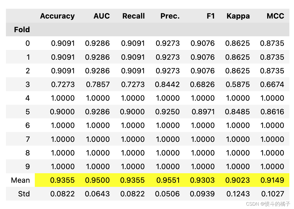
# 定义调参网格
dt_grid = {'max_depth' : [None, 2, 4, 6, 8, 10, 12]}

# 使用自定义网格和优化指标为F1来调整模型
tuned_dt = tune_model(dt, custom_grid = dt_grid, optimize = 'F1')

在这里插入图片描述

Processing:   0%|          | 0/7 [00:00<?, ?it/s]


Fitting 10 folds for each of 7 candidates, totalling 70 fits

# 使用tune_model函数对决策树模型进行调参
# 返回调参后的决策树模型和调参器对象
tuned_dt, tuner = tune_model(dt, return_tuner=True)

# 注意：为了访问调参器对象，需要将return_tuner参数设置为True

在这里插入图片描述

Processing:   0%|          | 0/7 [00:00<?, ?it/s]


Fitting 10 folds for each of 10 candidates, totalling 100 fits

# 创建一个决策树模型对象

tuned_dt

请添加图片描述

# 创建一个tuner对象

# tuner object
tuner

请添加图片描述

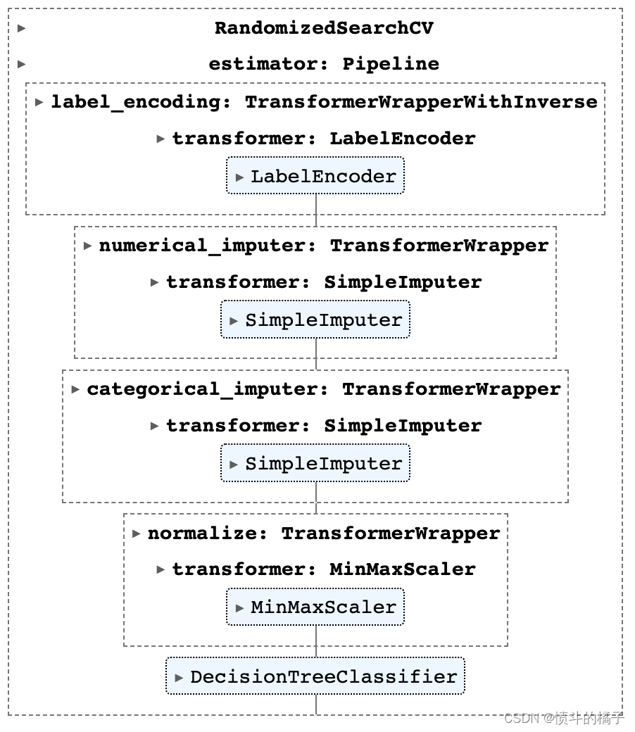
默认的搜索算法是sklearn中的RandomizedSearchCV。可以通过使用search_library和search_algorithm参数来进行更改。

# 使用Optuna库来调整决策树模型（dt）
# 调整后的模型保存在tuned_dt中
tuned_dt = tune_model(dt, search_library='optuna')

在这里插入图片描述

Processing:   0%|          | 0/7 [00:00<?, ?it/s]


[32m[I 2023-02-16 14:39:11,277][0m Searching the best hyperparameters using 105 samples...[0m
[32m[I 2023-02-16 14:39:18,586][0m Finished hyperparemeter search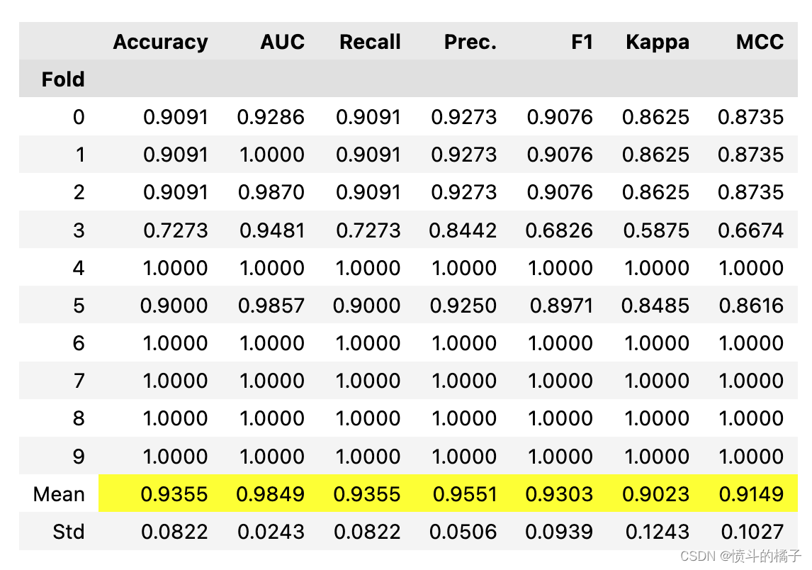![0m

有关所有可用的search_library和search_algorithm的更多详细信息，请查看docstring。在tune_model中，您可能会发现一些其他非常有用的参数：

choose_better
n_iter
early_stopping
groups

您可以查看函数的docstring以获取更多信息。

# help(tune_model)

✅ 集成模型

该函数对给定的估计器进行集成。该函数的输出是一个包含按折叠计算的CV分数的评分网格。可以使用get_metrics函数访问在CV期间评估的指标。可以使用add_metric和remove_metric函数添加或删除自定义指标。

# 使用Bagging方法对决策树模型dt进行集成
ensemble_model(dt, method='Bagging')

在这里插入图片描述

Processing:   0%|          | 0/6 [00:00<?, ?it/s]

请添加图片描述

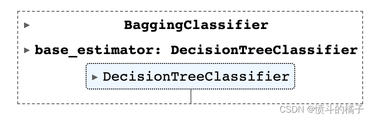
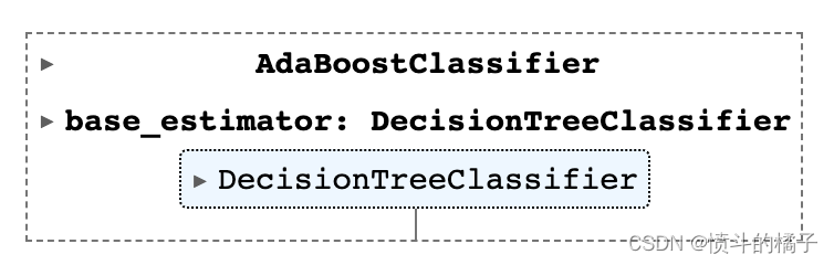
# 调用ensemble_model函数，传入决策树模型dt和方法参数为'Boosting'
ensemble_model(dt, method='Boosting')

在这里插入图片描述

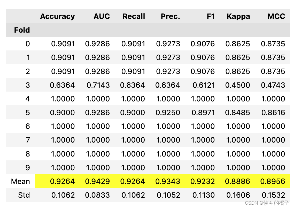
Processing:   0%|          | 0/6 [00:00<?, ?it/s]

请添加图片描述

一些在ensemble_model中可能非常有用的其他参数包括：

choose_better
n_estimators
groups
fit_kwargs
probability_threshold
return_train_score

您可以查看函数的文档字符串以获取更多信息。

# help(ensemble_model)

✅ 混合模型

该函数用于训练一个软投票/多数规则分类器，该分类器选择在estimator_list参数中传递的模型。该函数的输出是一个带有交叉验证分数的评分网格。可以使用get_metrics函数访问在CV期间评估的指标。可以使用add_metric和remove_metric函数添加或删除自定义指标。

# 定义一个变量best_recall_models_top3，用于存储基于召回率的前三个模型的信息
best_recall_models_top3

[QuadraticDiscriminantAnalysis(priors=None, reg_param=0.0,
                               store_covariance=False, tol=0.0001),
 LinearDiscriminantAnalysis(covariance_estimator=None, n_components=None,
                            priors=None, shrinkage=None, solver='svd',
                            store_covariance=False, tol=0.0001),
 KNeighborsClassifier(algorithm='auto', leaf_size=30, metric='minkowski',
                      metric_params=None, n_jobs=-1, n_neighbors=5, p=2,
                      weights='uniform')]

# blend_models函数用于将最佳召回率的前三个模型进行融合

# 参数best_recall_models_top3是一个包含最佳召回率的前三个模型的列表

# 代码调用blend_models函数，并传入参数best_recall_models_top3，将返回值赋给变量blend_models

blend_models(best_recall_models_top3)

在这里插入图片描述

Processing:   0%|          | 0/6 [00:00<?, ?it/s]

请添加图片描述

一些在blend_models中可能非常有用的其他参数包括：

choose_better
method
weights
fit_kwargs
probability_threshold
return_train_score

您可以查看函数的文档字符串以获取更多信息。

# help(blend_models)

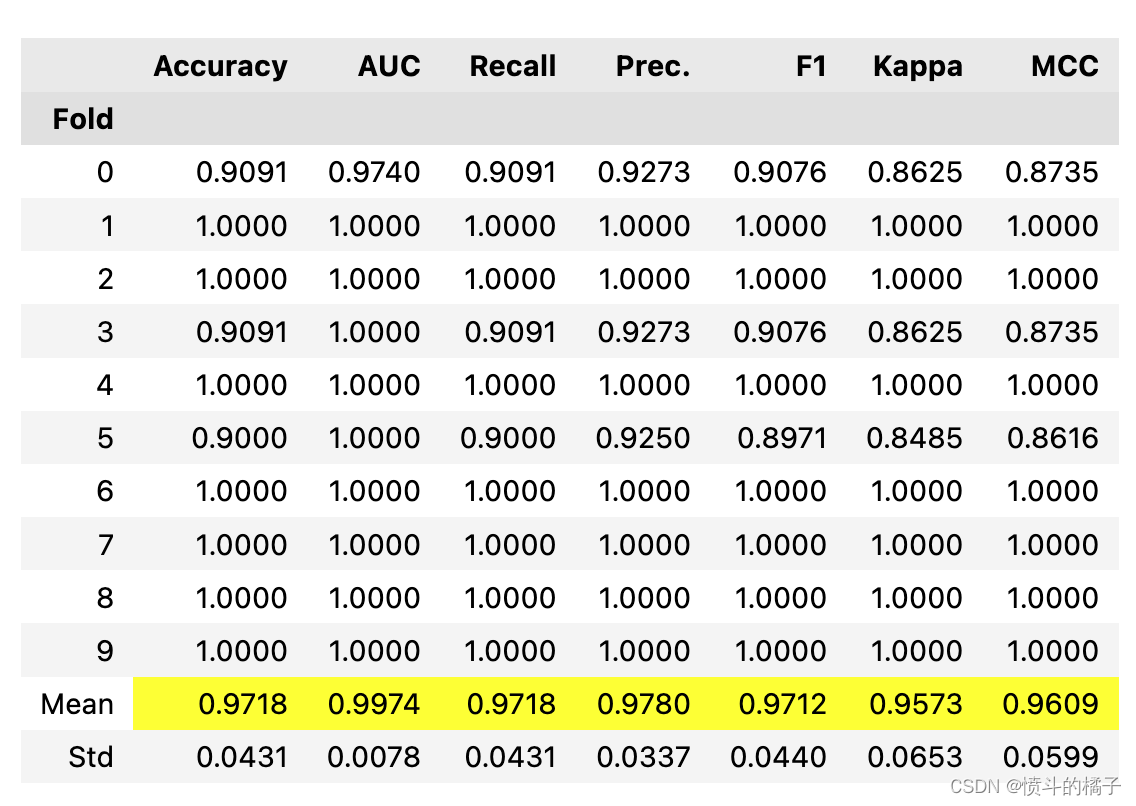
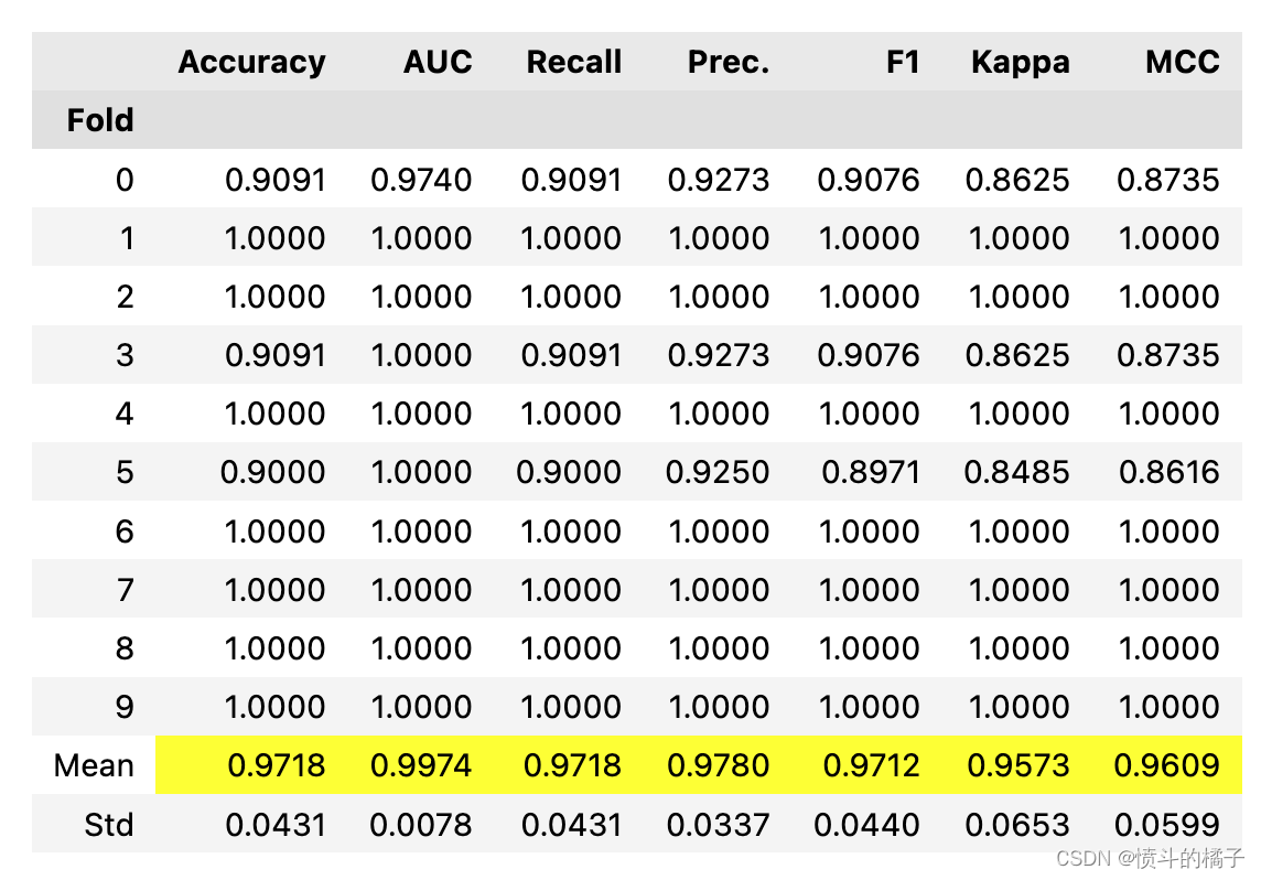
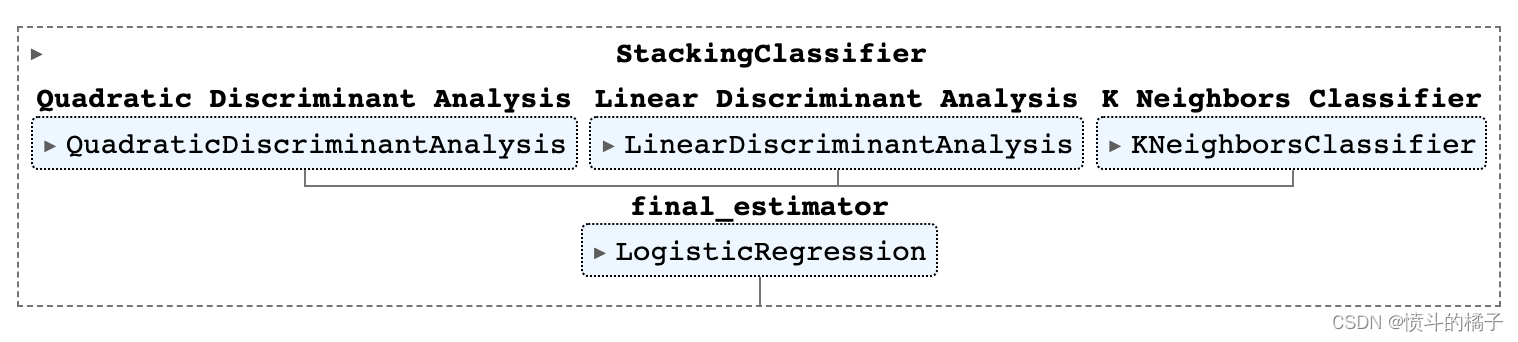
✅ 堆叠模型

该函数在estimator_list参数中传递的选择的估计器上训练一个元模型。该函数的输出是一个包含每个折叠的CV分数的评分网格。可以使用get_metrics函数访问CV期间评估的指标。可以使用add_metric和remove_metric函数添加或删除自定义指标。

# stack_models函数用于堆叠多个模型

# 参数：
# best_recall_models_top3：一个包含了最佳召回率的前三个模型的列表

# 算法流程：
# 1. 创建一个新的模型，用于堆叠多个模型
# 2. 将best_recall_models_top3列表中的模型添加到新的模型中
# 3. 返回堆叠后的模型
stack_models(best_recall_models_top3)

在这里插入图片描述

Processing:   0%|          | 0/6 [00:00<?, ?it/s]

请添加图片描述

一些在stack_models中可能非常有用的其他参数包括：

choose_better
meta_model
method
restack
probability_threshold
return_train_score

您可以查看函数的文档字符串以获取更多信息。

# help(stack_models)

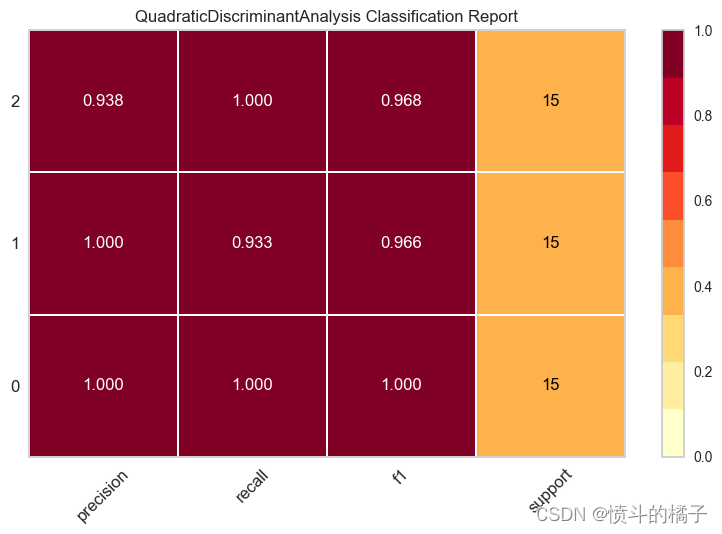
✅ 绘制模型

功能说明

该函数用于分析在保留集上训练模型的性能。在

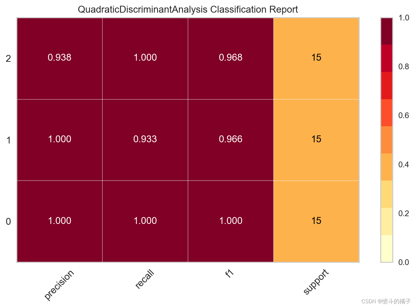
# plot class report
plot_model(best, plot = 'class_report')

在这里插入图片描述


# 绘制模型的分类报告图表
# 参数best表示要绘制的模型
# 参数plot表示要绘制的图表类型，这里选择分类报告图表
# 参数scale表示图表的缩放比例，这里选择缩放比例为2
plot_model(best, plot='class_report', scale=2)

在这里插入图片描述

# 导入所需的库
import matplotlib.pyplot as plt
from sklearn.metrics import classification_report

# 绘制分类报告图表并保存
# 参数best为模型对象
# 参数plot为要绘制的图表类型，这里选择'class_report'表示绘制分类报告图表
# 参数save为是否保存图表，这里设置为True表示保存图表
plot_model(best, plot = 'class_report', save=True)

'Class Report.png'

一些在plot_model中可能非常有用的其他参数包括：

fit_kwargs
plot_kwargs
groups
display_format

您可以查看函数的文档字符串以获取更多信息。

# help(plot_model)

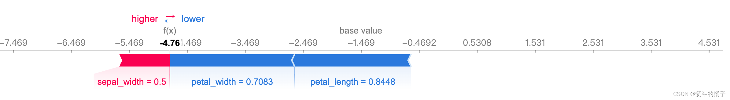
✅ 解释模型

该函数分析训练模型生成的预测结果。该函数中的大多数图表是基于SHAP（Shapley Additive exPlanations）实现的。有关更多信息，请参阅https://shap.readthedocs.io/en/latest/

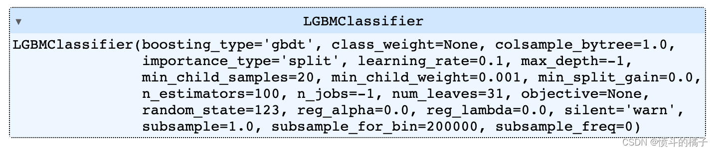
# 使用'lightgbm'算法创建一个分类模型
lightgbm = create_model('lightgbm')

在这里插入图片描述

Processing:   0%|          | 0/4 [00:00<?, ?it/s]

# 使用interpret_model函数对模型进行解释
# 参数lightgbm表示使用的模型是lightgbm模型
# 参数plot表示是否绘制模型的摘要图，默认为True
interpret_model(lightgbm, plot='summary')

在这里插入图片描述

# 使用interpret_model函数来解释lightgbm模型
# 参数plot='reason'表示绘制解释图表，observation=1表示解释测试集中的第一个观察值
interpret_model(lightgbm, plot='reason', observation=1)

在这里插入图片描述

一些在interpret_model中可能非常有用的其他参数包括：

plot
feature
use_train_data
X_new_sample
y_new_sample
save

您可以查看函数的文档字符串以获取更多信息。

# help(interpret_model)

✅ 获取排行榜

该函数返回当前设置中所有训练模型的排行榜。

# 获取排行榜
lb = get_leaderboard()
lb

Processing:   0%|          | 0/58 [00:00<?, ?it/s]

在这里插入图片描述

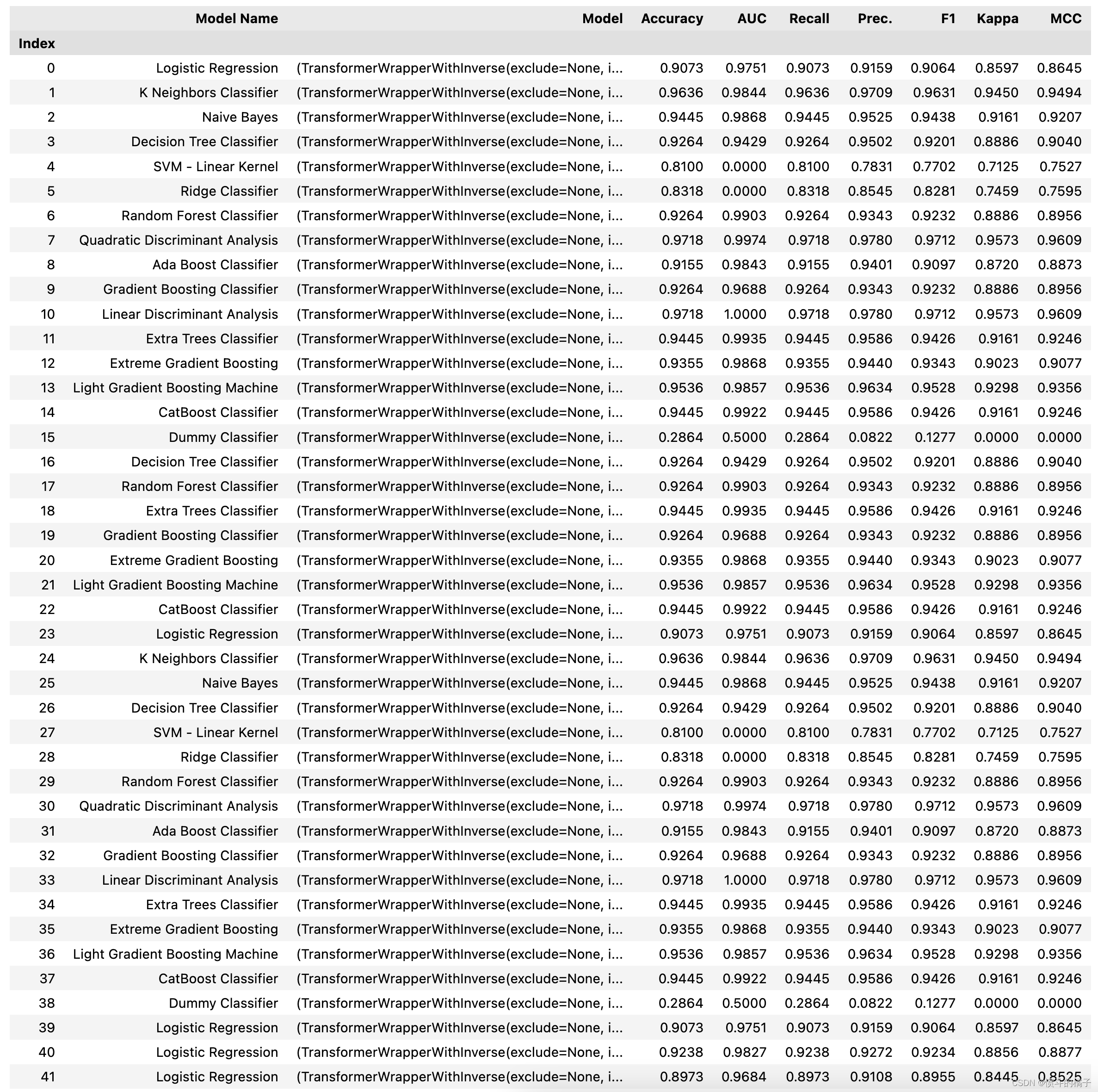
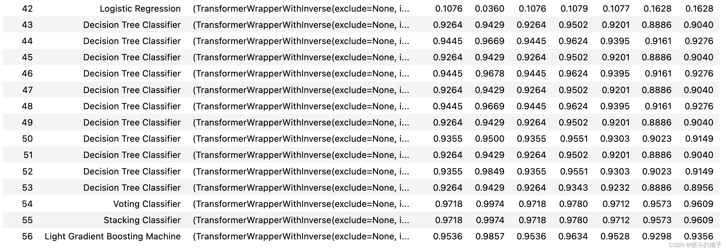
# 根据F1值选择最佳模型
# 使用sort_values方法对数据框lb按照F1列进行降序排序
# 使用['Model']索引获取排序后的数据框的Model列
# 使用iloc[0]获取排序后的Model列的第一个元素，即F1值最高的模型名称
lb.sort_values(by='F1', ascending=False)['Model'].iloc[0]

请添加图片描述

一些在get_leaderboard中可能非常有用的其他参数包括：

finalize_models
fit_kwargs
model_only
groups

您可以查看函数的docstring以获取更多信息。

# help(get_leaderboard)

✅ AutoML

该函数根据优化参数返回当前设置中所有训练模型中的最佳模型。可以使用get_metrics函数访问评估的指标。

automl()

请添加图片描述

✅ 仪表盘

仪表盘功能用于为训练模型生成交互式仪表盘。该仪表盘是使用ExplainerDashboard实现的。更多信息请查看Explainer Dashboard.

# 定义一个名为dashboard的函数
# 参数dt表示数据表，display_format表示显示格式，默认为'inline'

# 函数功能：用于显示数据表的仪表板

# 参数说明：
# - dt: 数据表，即要显示的数据
# - display_format: 显示格式，可以是'inline'或者其他格式，默认为'inline'

# 返回值：无

# 代码实现：
# 通过调用dashboard函数，可以将数据表以指定的显示格式显示在仪表板上。默认情况下，数据表以'inline'格式显示。
dashboard(dt, display_format ='inline')

Note: model_output=='probability', so assuming that raw shap output of DecisionTreeClassifier is in probability space...
Generating self.shap_explainer = shap.TreeExplainer(model)
Building ExplainerDashboard..
The explainer object has no decision_trees property. so setting decision_trees=False...
Warning: calculating shap interaction values can be slow! Pass shap_interaction=False to remove interactions tab.
Generating layout...
Calculating shap values...
Calculating prediction probabilities...
Calculating metrics...
Calculating confusion matrices...
Calculating classification_dfs...
Calculating roc auc curves...
Calculating pr auc curves...
Calculating liftcurve_dfs...
Calculating shap interaction values... (this may take a while)
Reminder: TreeShap computational complexity is O(TLD^2), where T is the number of trees, L is the maximum number of leaves in any tree and D the maximal depth of any tree. So reducing these will speed up the calculation.
Calculating dependencies...
Calculating permutation importances (if slow, try setting n_jobs parameter)...
Calculating pred_percentiles...
Calculating predictions...
Reminder: you can store the explainer (including calculated dependencies) with explainer.dump('explainer.joblib') and reload with e.g. ClassifierExplainer.from_file('explainer.joblib')
Registering callbacks...
Starting ExplainerDashboard inline (terminate it with ExplainerDashboard.terminate(8050))

✅创建应用程序

此函数创建一个用于推理的基本 gradio 应用程序。

# 创建一个Gradio应用

# 参数：
# - best: 一个模型或函数，用于处理输入并生成输出

create_app(best)  # 调用create_app函数，传入参数best，用于创建一个Gradio应用

Running on local URL:  http://127.0.0.1:7860

To create a public link, set `share=True` in `launch()`.

✅ 创建API

该函数接受一个输入模型，并创建一个用于推理的POST API。

# 创建API
# 参数：
# - best: 最佳模型
# - api_name: API的名称，默认为'my_first_api'
create_api(best, api_name='my_first_api')

API successfully created. This function only creates a POST API, it doesn't run it automatically. To run your API, please run this command --> !python my_first_api.py

# 导入必要的库
from flask import Flask, request, jsonify

# 创建一个Flask应用
app = Flask(__name__)

# 创建一个路由，用于处理POST请求
@app.route('/api', methods=['POST'])
def my_api():
    # 获取请求中的数据
    data = request.get_json()

    # 从请求数据中获取名字
    name = data['name']

    # 从请求数据中获取年龄
    age = data['age']

    # 计算出出生年份
    birth_year = 2021 - int(age)

    # 构建响应数据
    response = {
        'name': name,
        'birth_year': birth_year
    }

    # 返回响应数据
    return jsonify(response)

# 运行应用
if __name__ == '__main__':
    app.run()

# 导入必要的库
import flask
from flask import request, jsonify

# 创建一个Flask应用
app = flask.Flask(__name__)

# 设置应用的路由
@app.route('/', methods=['GET'])
def home():
    return "<h1>Welcome to my first API!</h1>"

# 设置应用的路由
@app.route('/api', methods=['GET'])
def api():
    # 创建一个字典
    data = {'name': 'John', 'age': 30, 'city': 'New York'}
    # 将字典转换为JSON格式
    return jsonify(data)

# 运行应用
if __name__ == '__main__':
    app.run(debug=True)

✅ 创建Docker

该函数用于创建用于将API端点投入生产的Dockerfile和requirements.txt文件。

# 定义一个函数create_docker，用于创建一个名为'my_first_api'的Docker容器
def create_docker(name):
    # 导入所需的模块
    import docker
    
    # 创建一个Docker客户端对象
    client = docker.from_env()
    
    # 检查是否存在同名的容器
    if name in [container.name for container in client.containers.list()]:
        # 如果存在同名容器，则打印提示信息并返回
        print("容器已存在")
        return
    
    # 创建一个新的容器
    container = client.containers.create(
        image='ubuntu:latest',  # 使用最新版本的Ubuntu镜像
        name=name,  # 设置容器的名称为传入的参数name
        detach=True  # 在后台运行容器
    )
    
    # 启动容器
    container.start()
    
    # 打印容器的ID和名称
    print(f"容器ID: {container.id}")
    print(f"容器名称: {container.name}")

Writing requirements.txt
Writing Dockerfile
Dockerfile and requirements.txt successfully created.
    To build image you have to run --> !docker image build -f "Dockerfile" -t IMAGE_NAME:IMAGE_TAG .

# 检查使用魔术命令创建的DockerFile文件

# 指定基础镜像为python:3.7
FROM python:3.7

# 设置工作目录为/app
WORKDIR /app

# 将当前目录下的所有文件复制到/app目录下
COPY . /app

# 安装依赖包
RUN pip install -r requirements.txt

# 设置环境变量
ENV FLASK_APP=app.py

# 暴露容器的端口号
EXPOSE 5000

# 运行flask应用
CMD ["flask", "run", "--host=0.0.0.0"]

# 检查使用魔术命令创建的requirements.txt文件

# 导入所需的模块
import os
import subprocess

# 定义一个函数，用于检查requirements.txt文件是否存在
def check_requirements_file():
    # 检查当前目录下是否存在requirements.txt文件
    if os.path.exists('requirements.txt'):
        print("requirements.txt文件已存在")
    else:
        print("requirements.txt文件不存在")

# 定义一个函数，用于安装requirements.txt文件中列出的所有依赖项
def install_requirements():
    # 检查当前目录下是否存在requirements.txt文件
    if os.path.exists('requirements.txt'):
        # 使用subprocess模块执行命令，安装requirements.txt文件中列出的所有依赖项
        subprocess.call(['pip', 'install', '-r', 'requirements.txt'])
        print("所有依赖项已成功安装")
    else:
        print("requirements.txt文件不存在，无法安装依赖项")

# 调用函数，检查requirements.txt文件是否存在
check_requirements_file()

# 调用函数，安装requirements.txt文件中列出的所有依赖项
install_requirements()

✅ 完善模型

该函数在整个数据集上训练给定的模型，包括保留集。

# 将模型进行最终化处理
final_best = finalize_model(best)

# 定义一个变量final_best，用于存储最终的最佳结果

final_best = None

请添加图片描述

✅ 转换模型

该函数将训练好的机器学习模型的决策函数转换为不同的编程语言，如Python、C、Java、Go、C#等。如果您想要将模型部署到无法安装正常Python堆栈以支持模型推断的环境中，这非常有用。

# 将学习到的函数转换为Java代码
# 调用convert_model函数，将决策树模型(dt)转换为Java代码
# 设置language参数为'java'，表示转换为Java语言的代码
# 打印输出转换后的Java代码结果

public class Model {
    public static double[] score(double[] input) {
        double[] var0;
        if (input[2] <= 0.23275858908891678) {
            var0 = new double[] {1.0, 0.0, 0.0};
        } else {
            if (input[2] <= 0.62931028008461) {
                if (input[0] <= 0.180555522441864) {
                    var0 = new double[] {0.0, 0.0, 1.0};
                } else {
                    var0 = new double[] {0.0, 1.0, 0.0};
                }
            } else {
                if (input[2] <= 0.6637930274009705) {
                    if (input[1] <= 0.3958333134651184) {
                        var0 = new double[] {0.0, 0.0, 1.0};
                    } else {
                        var0 = new double[] {0.0, 1.0, 0.0};
                    }
                } else {
                    if (input[3] <= 0.6666666269302368) {
                        if (input[3] <= 0.6041666567325592) {
                            var0 = new double[] {0.0, 0.0, 1.0};
                        } else {
                            if (input[0] <= 0.6388888359069824) {
                                var0 = new double[] {0.0, 1.0, 0.0};
                            } else {
                                var0 = new double[] {0.0, 0.0, 1.0};
                            }
                        }
                    } else {
                        var0 = new double[] {0.0, 0.0, 1.0};
                    }
                }
            }
        }
        return var0;
    }
}

✅ 部署模型

此函数在云上部署整个机器学习流程。

AWS: 在AWS S3上部署模型时，必须使用命令行界面配置环境变量。要配置AWS环境变量，请在终端中输入aws configure命令。以下信息是必需的，可以使用您的Amazon控制台帐户的身份和访问管理（IAM）门户生成：

AWS访问密钥ID
AWS秘密密钥访问
默认区域名称（可以在AWS控制台的全局设置下看到）
默认输出格式（必须留空）

GCP: 要在Google Cloud Platform（‘gcp’）上部署模型，必须使用命令行或GCP控制台创建项目。创建项目后，您必须创建一个服务帐户，并将服务帐户密钥下载为JSON文件，以在本地环境中设置环境变量。了解更多信息：https://cloud.google.com/docs/authentication/production

Azure: 要在Microsoft Azure（‘azure’）上部署模型，必须在本地环境中设置用于连接字符串的环境变量。转到Azure门户上的存储帐户设置以访问所需的连接字符串。
AZURE_STORAGE_CONNECTION_STRING（作为环境变量必需）
了解更多信息：https://docs.microsoft.com/en-us/azure/storage/blobs/storage-quickstart-blobs-python?toc=%2Fpython%2Fazure%2FTOC.json

# 在AWS S3上部署模型
# 部署模型函数deploy_model()用于将模型部署到AWS S3上
# 参数best表示要部署的模型
# 参数model_name表示在AWS上部署的模型的名称，这里设置为'my_first_platform_on_aws'
# 参数platform表示要部署到的平台，这里设置为'aws'
# 参数authentication是一个字典，用于身份验证
# 字典中的'bucket'表示要部署到的AWS S3存储桶的名称，这里设置为'pycaret-test'

# 从AWS S3加载模型
# 从AWS S3加载名为'my_first_platform_on_aws'的模型
# 使用AWS平台加载模型
# 鉴权信息为{'bucket' : 'pycaret-test'}
# 加载模型并赋值给loaded_from_aws变量

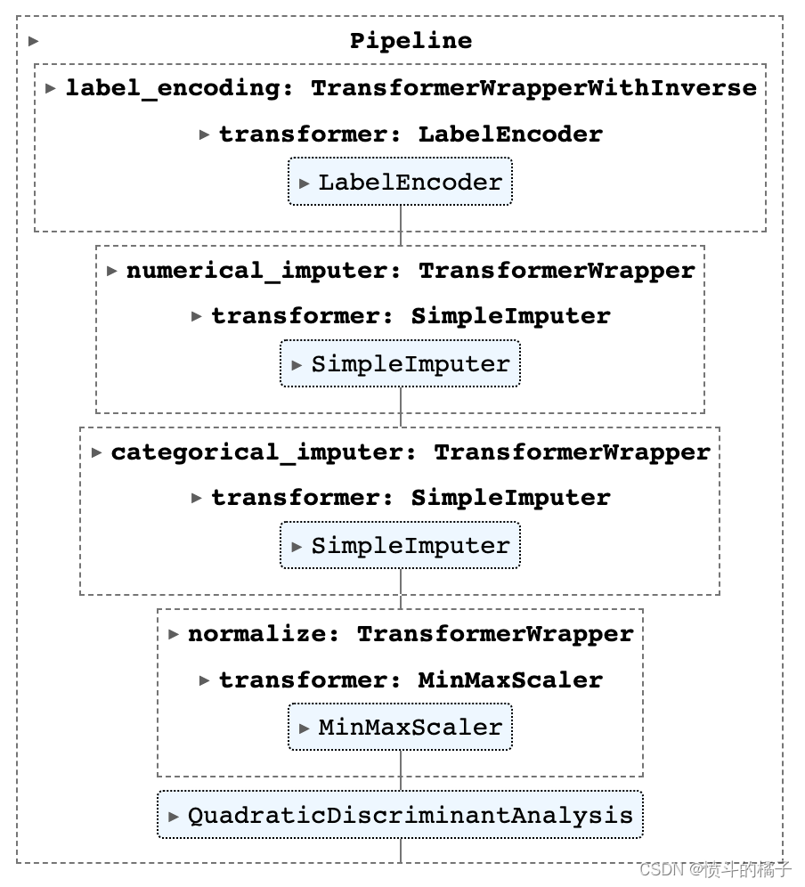
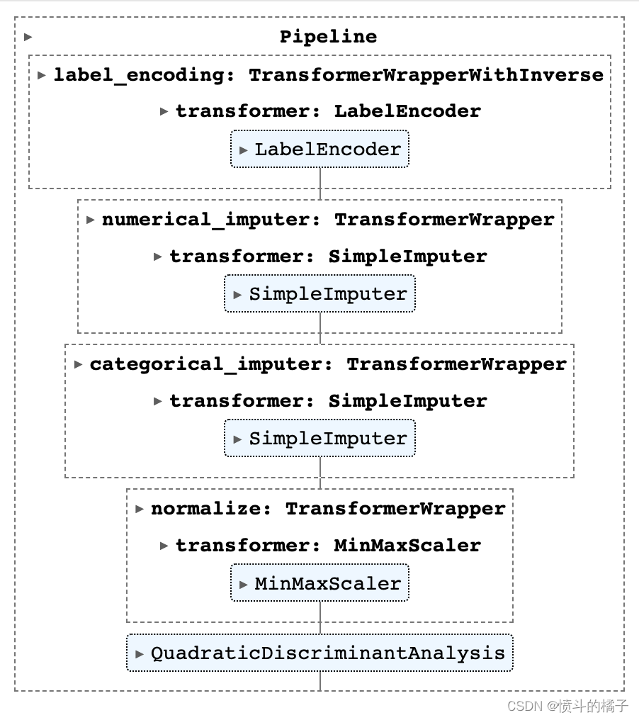
✅ 保存/加载模型

这个函数将转换流水线和训练好的模型对象保存到当前工作目录中，以pickle文件的形式供以后使用。

# 保存模型
# 使用save_model函数将最佳模型保存为'my_first_model'文件

Transformation Pipeline and Model Successfully Saved





(Pipeline(memory=FastMemory(location=C:\Users\owner\AppData\Local\Temp\joblib),
          steps=[('label_encoding',
                  TransformerWrapperWithInverse(exclude=None, include=None,
                                                transformer=LabelEncoder())),
                 ('numerical_imputer',
                  TransformerWrapper(exclude=None,
                                     include=['sepal_length', 'sepal_width',
                                              'petal_length', 'petal_width'],
                                     transformer=SimpleImputer(add_indicator=F...
                                     transformer=SimpleImputer(add_indicator=False,
                                                               copy=True,
                                                               fill_value=None,
                                                               missing_values=nan,
                                                               strategy='most_frequent',
                                                               verbose='deprecated'))),
                 ('normalize',
                  TransformerWrapper(exclude=None, include=None,
                                     transformer=MinMaxScaler(clip=False,
                                                              copy=True,
                                                              feature_range=(0,
                                                                             1)))),
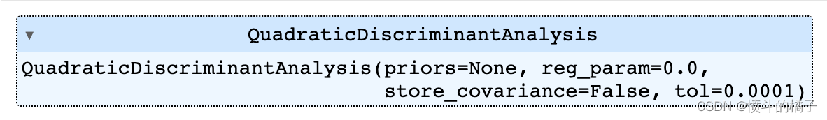
                 ('trained_model',
                  QuadraticDiscriminantAnalysis(priors=None, reg_param=0.0,
                                                store_covariance=False,
                                                tol=0.0001))],
          verbose=False),
 'my_first_model.pkl')

# 加载模型
loaded_from_disk = load_model('my_first_model')  # 从磁盘上加载名为'my_first_model'的模型文件，并将其存储在变量loaded_from_disk中
loaded_from_disk  # 打印加载的模型

Transformation Pipeline and Model Successfully Loaded

请添加图片描述

✅ 保存/加载实验

该函数将实验中的所有变量保存在磁盘上，以便以后恢复而无需重新运行设置函数。

# 保存实验
save_experiment('my_experiment')

# 从磁盘加载实验
exp_from_disk = load_experiment('my_experiment', data=data)

在这里插入图片描述

本代码链接：

https://download.csdn.net/download/wjjc1017/88643312

数智笔记

关注

23
点赞
踩
28

收藏

觉得还不错? 一键收藏
打赏
0
评论
工具系列：PyCaret介绍_多分类代码示例

这个函数在PyCaret中初始化实验，并根据传入函数的所有参数创建转换流水线。在执行任何其他函数之前，必须调用设置函数。data和target。所有其他参数都是可选的，并用于配置数据预处理流水线。# 设置数据集和目标变量# data: 数据集# target: 目标变量，即要预测的变量# session_id: 用于重现实验结果的随机种子要访问由设置函数创建的所有变量，例如转换后的数据集、随机状态等，您可以使用get_config方法。# 获取所有可用的配置信息 get_config()
复制链接

扫一扫