


Python优雅地绘制北半球投影地图
经常在Nature正刊和子刊中看到北半球或南半球投影的球形地图,非常美观~
这种图ArcGIS往往不方便绘制
在子刊***Nat. Clim. Chang.***中,通过北极俯视投影表示NAO和AO的EOF分解。
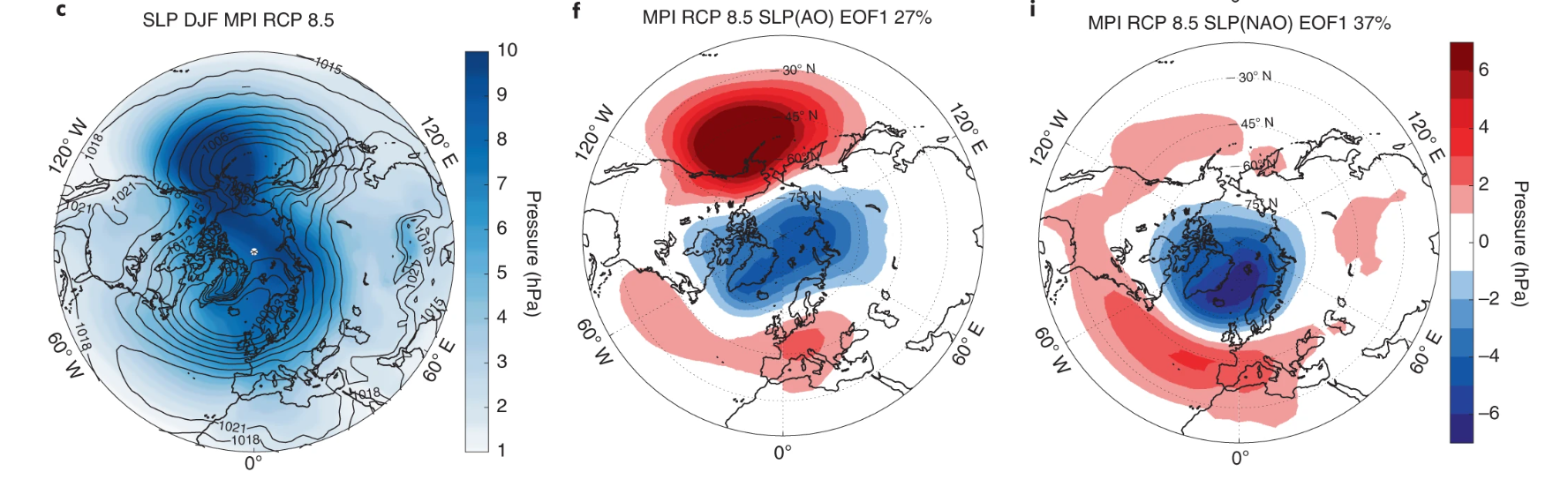
Hamouda, M.E., Pasquero, C. & Tziperman, E. Decoupling of the Arctic Oscillation and North Atlantic Oscillation in a warmer climate. Nat. Clim. Chang. 11, 137–142 (2021). https://doi.org/10.1038/s41558-020-00966-8
如子刊Nature Geosci中表示了海冰的漂移,还添加了DEM底图,非常美观。
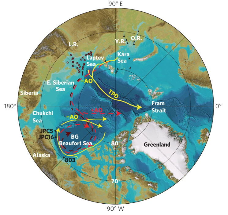
Darby, D., Ortiz, J., Grosch, C. et al. 1,500-year cycle in the Arctic Oscillation identified in Holocene Arctic sea-ice drift. Nature Geosci 5, 897–900 (2012). https://doi.org/10.1038/ngeo1629
接下来让我们复现一下试试
数据
以海温数据为例,ERA5月温度平均,是一张721*1440的0.25degTIF
import rioxarray as rxr
file_name='/home/mw/project/SST.tif'
ds=rxr.open_rasterio(file_name)
data = ds[0]
如果你有其它nc数据,也可以通过xarray读取
投影设置
其实cartopy提供了一些投影使用
如AzimuthalEquidistant
这是一种等距方位投影,是指使图上面积和相应的实际地面面积相等的方位投影,分为正轴,横轴、斜轴投影。其中纬线为同心圆弧,经线为圆的半径。该投影提供了围绕中心位置的精确角度和距离。其他角度、距离或区域可能会变形。
北半球的投影叫做AzimuthalEquidistant cartopy的投影列表是有这个投影的: https://scitools.org.uk/cartopy/docs/latest/reference/projections.html 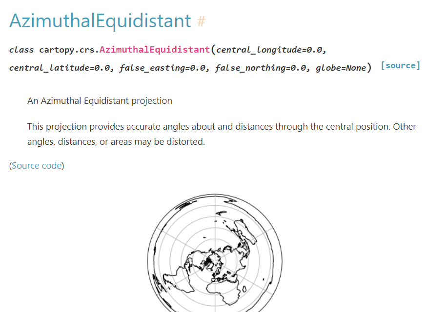
import matplotlib.pyplot as plt
import cartopy.crs as ccrs
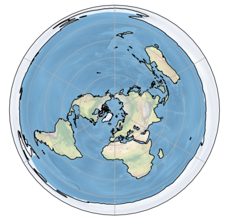
plt.figure(figsize=(6, 6))
ax = plt.axes(projection=ccrs.AzimuthalEquidistant(central_latitude=90))
ax.coastlines()
ax.gridlines()
ax.stock_img()
绘图代码
接下来我们把数据添加
import matplotlib.pyplot as plt
import cartopy.crs as ccrs
import numpy as np
import cartopy.feature as cfeature
import matplotlib.path as mpath
import mplotutils as mpu
from utils import plot

fig = plt.figure()

proj=ccrs.AzimuthalEquidistant(central_latitude=90)
ax = fig.add_subplot(111, projection=proj)
levels = np.linspace(270, 300, num=31)
data_renamed = data.rename({'x': 'lon', 'y': 'lat'})
h = plot.one_map_flat(data_renamed, ax, levels=levels, cmap="BrBG_r", mask_ocean=False, add_coastlines=True, add_land=False, plotfunc="contourf")
其中plot.one_map_flat是我之前撰写的绘图函数,感兴趣的同学可见相关推送
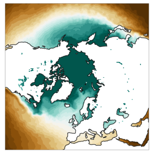
现在的结果看起来不错,但太大了,我们如果只需要北半球的数据,则需要指定经纬度。
我们使用ax.set_extent([-180, 180, 30, 90])将经纬度指定在30°-90°
import matplotlib.pyplot as plt
import cartopy.crs as ccrs
import numpy as np
import cartopy.feature as cfeature
import matplotlib.path as mpath
import mplotutils as mpu

fig = plt.figure()

proj=ccrs.AzimuthalEquidistant(central_latitude=90)
ax = fig.add_subplot(111, projection=proj)
levels = np.linspace(270, 300, num=31)
data_renamed = data.rename({'x': 'lon', 'y': 'lat'})
h = plot.one_map_flat(data_renamed, ax, levels=levels, cmap="BrBG_r", mask_ocean=False, add_coastlines=True, add_land=False, plotfunc="contourf")

ax.set_extent([-180, 180, 30, 90], crs=ccrs.PlateCarree())
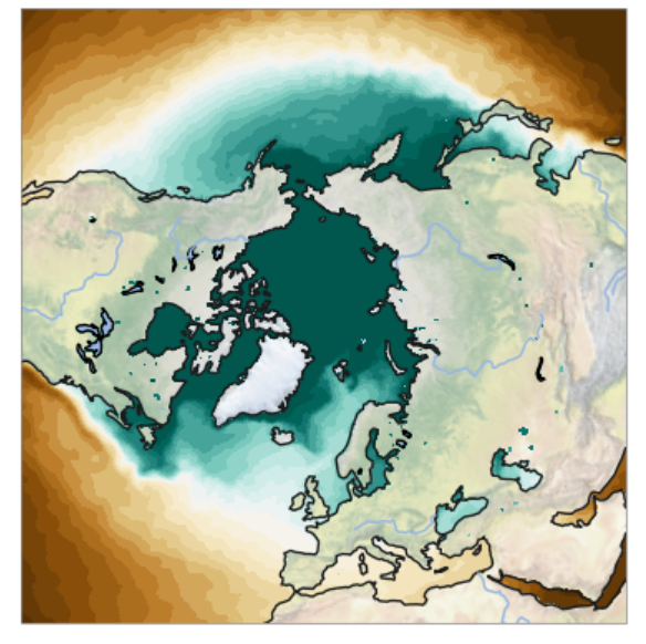
再次添加更多要素:
import matplotlib.pyplot as plt
import cartopy.crs as ccrs
import numpy as np
import cartopy.feature as cfeature
import matplotlib.path as mpath
import mplotutils as mpu

fig = plt.figure()

proj=ccrs.AzimuthalEquidistant(central_latitude=90)
ax = fig.add_subplot(111, projection=proj)
levels = np.linspace(270, 300, num=31)
data_renamed = data.rename({'x': 'lon', 'y': 'lat'})
h = plot.one_map_flat(data_renamed, ax, levels=levels, cmap="BrBG_r", mask_ocean=False, add_coastlines=True, add_land=False, plotfunc="contourf")

ax.set_extent([-180, 180, 30, 90], crs=ccrs.PlateCarree())

ax.add_feature(cfeature.OCEAN)
ax.add_feature(cfeature.LAND, edgecolor='black')
ax.add_feature(cfeature.LAKES, edgecolor='black')
ax.add_feature(cfeature.RIVERS)
ax.stock_img()
-
proj=ccrs.AzimuthalEquidistant(central_latitude=90), ax = plt.axes(projection=proj)仅在定义图层的时候设置为该投影,其余设置content,绘制contourf都是PlateCaree -
绘制完结果也是正方形,和ArcGIS差不多,见之前的推文 -
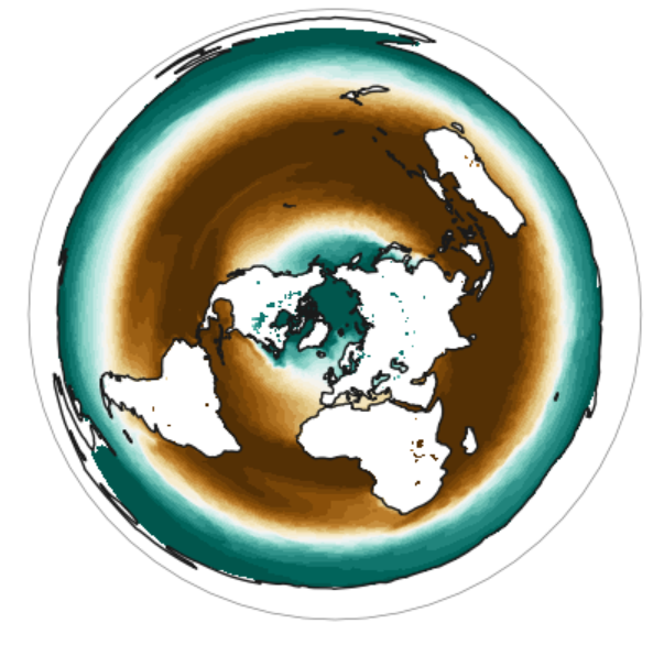
cartopy灵活的地方在于适配matplotlib,因此可以设置一圆形进行相交:
import matplotlib.pyplot as plt
import cartopy.crs as ccrs
import numpy as np
import cartopy.feature as cfeature
import matplotlib.path as mpath
import mplotutils as mpu

fig = plt.figure()

proj=ccrs.AzimuthalEquidistant(central_latitude=90)
ax = fig.add_subplot(111, projection=proj)
levels = np.linspace(270, 300, num=31)
data_renamed = data.rename({'x': 'lon', 'y': 'lat'})
h = plot.one_map_flat(data_renamed, ax, levels=levels, cmap="BrBG_r", mask_ocean=False, add_coastlines=True, add_land=False, plotfunc="contourf")

ax.set_extent([-180, 180, 30, 90], crs=ccrs.PlateCarree())
ax.add_feature(cfeature.OCEAN)
ax.add_feature(cfeature.LAND, edgecolor='black')
ax.add_feature(cfeature.LAKES, edgecolor='black')
ax.add_feature(cfeature.RIVERS)
ax.stock_img()

theta = np.linspace(0, 2*np.pi, 100)
center, radius = [0.5, 0.5], 0.5
verts = np.vstack([np.sin(theta), np.cos(theta)]).T
circle = mpath.Path(verts * radius + center)
# 将该Path设置为GeoAxes的边界
ax.set_boundary(circle, transform=ax.transAxes)

cbar = mpu.colorbar(
    h, ax1=ax, size=0.05, #height
            shrink=0.05, #width
            pad=0.1, orientation='horizontal'
)

cbar.ax.tick_params(labelsize='small')
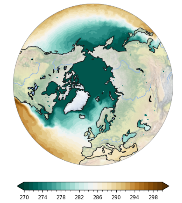
现在的结果相当不错了,只需要设置一下经纬度线
import matplotlib.pyplot as plt
import cartopy.crs as ccrs
import numpy as np
import cartopy.feature as cfeature
import matplotlib.path as mpath
import mplotutils as mpu

fig = plt.figure()

proj=ccrs.AzimuthalEquidistant(central_latitude=90)
ax = fig.add_subplot(111, projection=proj)
levels = np.linspace(270, 300, num=31)
data_renamed = data.rename({'x': 'lon', 'y': 'lat'})
h = plot.one_map_flat(data_renamed, ax, levels=levels, cmap="BrBG_r", mask_ocean=False, add_coastlines=True, add_land=False, plotfunc="contourf")


ax.set_extent([-180, 180, 30, 90], crs=ccrs.PlateCarree())
# 添加各种特征
ax.add_feature(cfeature.OCEAN)
ax.add_feature(cfeature.LAND, edgecolor='black')
ax.add_feature(cfeature.LAKES, edgecolor='black')
ax.add_feature(cfeature.RIVERS)
#ax.add_feature(cfeature.BORDERS)
ax.stock_img()

theta = np.linspace(0, 2*np.pi, 100)
center, radius = [0.5, 0.5], 0.5
verts = np.vstack([np.sin(theta), np.cos(theta)]).T
circle = mpath.Path(verts * radius + center)
# 将该Path设置为GeoAxes的边界
ax.set_boundary(circle, transform=ax.transAxes)

cbar = mpu.colorbar(
    h, ax1=ax, size=0.05, #height
            shrink=0.05, #width
            pad=0.1, orientation='horizontal'
)

cbar.ax.tick_params(labelsize='small')

gls = ax.gridlines(draw_labels=True, crs=ccrs.PlateCarree(),
                   color='k', linestyle='dashed', linewidth=0.3,
                   dms=True, x_inline=False, y_inline=False,
                   xlocs=np.arange(-180, 180 + 60, 60), ylocs=np.arange(0, 90 + 15, 15)
                  )

非常完美
感兴趣的同学可以后台回复【北半球】下载数据和代码


 1万+
1万+

 被折叠的 条评论
为什么被折叠?
被折叠的 条评论
为什么被折叠?
 到【灌水乐园】发言


