深度学习——优化算法

为什么需要优化算法

优化算法可以加快收敛速度（未加入优化的神经网络训练时间比加入优化后时间更短），甚至得到一个更好更小的损失函数值。优化算法能帮你快速高效地训练模型。

有哪些优化算法

• Mini-Batch 梯度下降
• Momentum 动量梯度下降法
• RMSprop
• Adam 提升算法

其中Adam提升算法是Momentum和RMSprop两种相结合的算法，接下来我们会依次介绍这四种算法。

Mini-Batch 梯度下降

算法介绍

训练集被分割为小的子训练集，这些子训练集被称为mini-batch。假设每个子集只有1000个训练数据，那么先取前1000个开始训练（训练方法与梯度下降完全相同，不同的只是对训练集进行了分割），再取接下来的1000个继续训练，依次类推，直到训练完所有的训练数据。以mini-batch为64为例，过程如下图所示：

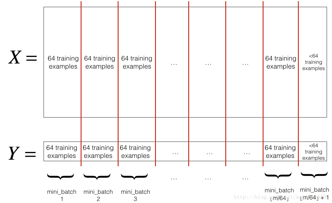
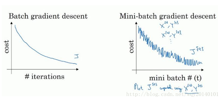
特别的，当每个mini-batch的大小为1时，得到一种新算法，叫做随机梯度下降，此时每次只取一个样本进行训练，效率过于低下，会失去向量化带来的加速。当mini-batch的大小为训练数据本身时，得到batch梯度下降，也就是我们普通的梯度下降算法（此时损失函数关于迭代次数的图像上，应该是一个持续下降的曲线，如果有上升的情况，那就是学习速率过大）

三种不同mini-batch代码对比

以下代码来自吴恩达coursera《deep learning》课后编程作业
- (Batch) Gradient Descent:

X = data_input
Y = labels
parameters = initialize_parameters(layers_dims)
for i in range(0, num_iterations):
    # Forward propagation
    a, caches = forward_propagation(X, parameters)
    # Compute cost.
    cost = compute_cost(a, Y)
    # Backward propagation.
    grads = backward_propagation(a, caches, parameters)
    # Update parameters.
    parameters = update_parameters(parameters, grads)

• Stochastic Gradient Descent:

X = data_input
Y = labels
parameters = initialize_parameters(layers_dims)
for i in range(0, num_iterations):
    for j in range(0, m):
        # Forward propagation
        a, caches = forward_propagation(X[:,j], parameters)
        # Compute cost
        cost = compute_cost(a, Y[:,j])
        # Backward propagation
        grads = backward_propagation(a, caches, parameters)
        # Update parameters.
        parameters = update_parameters(parameters, grads)

• Mini-batch Gradient Descent:

X = data_input
Y = labels
parameters = initialize_parameters(layers_dims)
for i in range(0, num_iterations):
     for minibatch in minibatches:
        # Select a minibatch
        (minibatch_X, minibatch_Y) = minibatch

        # Forward propagation
        a3, caches = forward_propagation(minibatch_X, parameters)
        # Compute cost
        cost = compute_cost(a3, minibatch_Y)

        # Backward propagation
        grads = backward_propagation(minibatch_X, minibatch_Y, caches)
        # Update parameters.
        parameters = update_parameters_with_gd(parameters, grads, learning_rate)

所以，我们的目标是找一个大小适中的mini-batch。

mini-batch选取数据集代码实现

# GRADED FUNCTION: random_mini_batches

def random_mini_batches(X, Y, mini_batch_size = 64, seed = 0):
    """
    Creates a list of random minibatches from (X, Y)

    Arguments:
    X -- input data, of shape (input size, number of examples)
    Y -- true "label" vector (1 for blue dot / 0 for red dot), of shape (1, number of examples)
    mini_batch_size -- size of the mini-batches, integer

    Returns:
    mini_batches -- list of synchronous (mini_batch_X, mini_batch_Y)
    """

    np.random.seed(seed)            # To make your "random" minibatches the same as ours
    m = X.shape[1]                  # number of training examples
    mini_batches = []

    # Step 1: Shuffle (X, Y)
    permutation = list(np.random.permutation(m))
    shuffled_X = X[:, permutation]
    shuffled_Y = Y[:, permutation].reshape((1,m))

    # Step 2: Partition (shuffled_X, shuffled_Y). Minus the end case.
    num_complete_minibatches = math.floor(m/mini_batch_size) # number of mini batches of size mini_batch_size in your partitionning
    for k in range(0, num_complete_minibatches):
        mini_batch_X = shuffled_X[:, mini_batch_size*k : mini_batch_size*(k+1)]
        mini_batch_Y = shuffled_Y[:, mini_batch_size*k : mini_batch_size*(k+1)]
        mini_batch = (mini_batch_X, mini_batch_Y)
        mini_batches.append(mini_batch)

    # Handling the end case (last mini-batch < mini_batch_size)
    if m % mini_batch_size != 0:
        mini_batch_X = shuffled_X[:, mini_batch_size*num_complete_minibatches : m]
        mini_batch_Y = shuffled_Y[:, mini_batch_size*num_complete_minibatches : m]
        mini_batch = (mini_batch_X, mini_batch_Y)
        mini_batches.append(mini_batch)

    return mini_batches

Momentum 动量梯度下降法

算法介绍

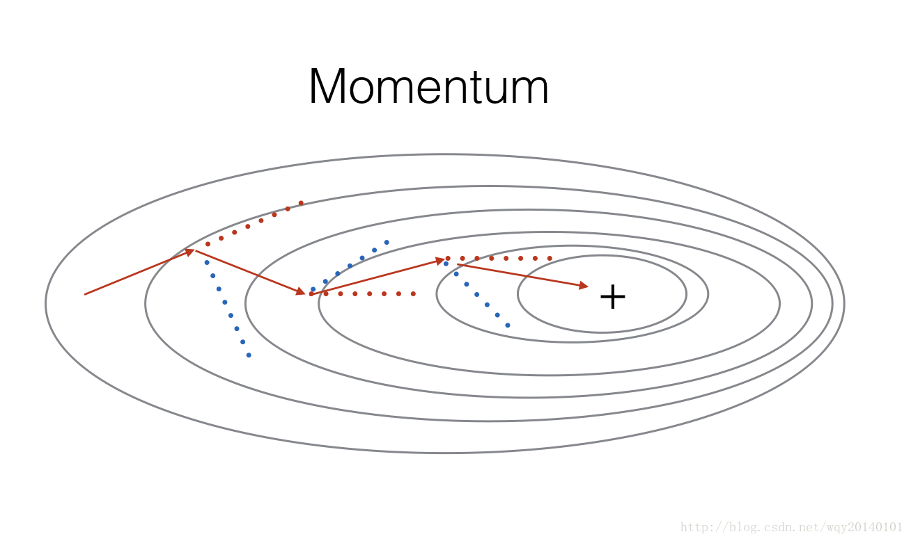
由于Mini-batch梯度下降使用数据子集进行参数更新，所以更新的方向跟普通的batch梯度下降有些不同，而是有一些变化（这里是指，不同的数据子集在进行梯度下降时，可能使损失函数值上升，但总趋势是下降的），因此小批量梯度下降的路径将会“震荡”到收敛。使用动量可以减少震荡。这些“变化“形象化表示如下：

动量梯度下降的公式如下：

$$\begin{cases} v_{dW^{[l]}} = \beta v_{dW^{[l]}} + (1 - \beta) dW^{[l]} \\ W^{[l]} = W^{[l]} - \alpha v_{dW^{[l]}} \end{cases}$$ $$\begin{cases} v_{db^{[l]}} = \beta v_{db^{[l]}} + (1 - \beta) db^{[l]} \\ b^{[l]} = b^{[l]} - \alpha v_{db^{[l]}} \end{cases}$$
其中 $\beta$ 是动量，一般设置为0.9， $\alpha$ 是学习速率。该公式蕴含这一种思想——指数加权平均。这里我不过多地从数学角度解释为什么这样，一个我个人认为易于理解的解释是，这种表达从图形化的角度来看，是把过去的梯度下降考虑在内来平滑当下的梯度变化，从而减小垂直方向上的震荡，同时保持水平方向上的下降速度。

代码实现

def update_parameters_with_momentum(parameters, grads, v, beta, learning_rate):
    """
    Update parameters using Momentum

    Arguments:
    parameters -- python dictionary containing your parameters:
                    parameters['W' + str(l)] = Wl
                    parameters['b' + str(l)] = bl
    grads -- python dictionary containing your gradients for each parameters:
                    grads['dW' + str(l)] = dWl
                    grads['db' + str(l)] = dbl
    v -- python dictionary containing the current velocity:
                    v['dW' + str(l)] = ...
                    v['db' + str(l)] = ...
    beta -- the momentum hyperparameter, scalar
    learning_rate -- the learning rate, scalar

    Returns:
    parameters -- python dictionary containing your updated parameters 
    v -- python dictionary containing your updated velocities
    """

    L = len(parameters) // 2 # number of layers in the neural networks

    # Momentum update for each parameter
    for l in range(L):
        # compute velocities
        v["dW" + str(l+1)] = beta*v["dW" + str(l+1)]+(1-beta)*grads["dW" + str(l+1)]
        v["db" + str(l+1)] =beta*v["db" + str(l+1)]+(1-beta)*grads["db" + str(l+1)]
        # update parameters
        parameters["W" + str(l+1)] = parameters["W" + str(l+1)]-learning_rate*v["dW" + str(l+1)]
        parameters["b" + str(l+1)] = parameters["b" + str(l+1)]-learning_rate*v["db" + str(l+1)]

    return parameters, v

RMSprop算法

算法介绍

与前一个算法的目的相同，我们想减少纵轴上的震荡，同时增大横纵上的收敛速度。我们推出跟前一个类似的公式：

$$s_{dW^{[l]}} = \beta_2 s_{dW^{[l]}} + (1 - \beta_2) (\frac{\partial \mathcal{J} }{\partial W^{[l]} })^2\\W^{[l]} = W^{[l]} - \alpha \frac{dW}{\sqrt{s_{dw^{[l]}}}}$$ 一个不太严谨的解释是，由于纵轴的震荡较大，即dw较大，s就会较大，当s被除后，使w变化较小。而横轴上下降较慢，同理推出运算后，使变化增大。

Adam算法

该算法是前两种算法的结合版本。公式如下：

$$\begin{cases} v_{dW^{[l]}} = \beta_1 v_{dW^{[l]}} + (1 - \beta_1) \frac{\partial \mathcal{J} }{ \partial W^{[l]} } \\ v^{corrected}_{dW^{[l]}} = \frac{v_{dW^{[l]}}}{1 - (\beta_1)^t} \\ s_{dW^{[l]}} = \beta_2 s_{dW^{[l]}} + (1 - \beta_2) (\frac{\partial \mathcal{J} }{\partial W^{[l]} })^2 \\ s^{corrected}_{dW^{[l]}} = \frac{s_{dW^{[l]}}}{1 - (\beta_1)^t} \\ W^{[l]} = W^{[l]} - \alpha \frac{v^{corrected}_{dW^{[l]}}}{\sqrt{s^{corrected}_{dW^{[l]}}} + \varepsilon} \end{cases}$$
- L is the number of layers
- $\beta_1$ and $\beta_2$ are hyperparameters that control the two exponentially weighted averages. 一般来说 $\beta_1$=0.9 $\beta_2$ =0.999我们的目标不是来调整这两个参数的。
- $\alpha$ is the learning rate
- $\varepsilon$ is a very small number to avoid dividing by zero 一般设为 $10^{-8}$

Adam更新参数的代码

def update_parameters_with_adam(parameters, grads, v, s, t, learning_rate = 0.01,
                                beta1 = 0.9, beta2 = 0.999,  epsilon = 1e-8):
    """
    Update parameters using Adam

    Arguments:
    parameters -- python dictionary containing your parameters:
                    parameters['W' + str(l)] = Wl
                    parameters['b' + str(l)] = bl
    grads -- python dictionary containing your gradients for each parameters:
                    grads['dW' + str(l)] = dWl
                    grads['db' + str(l)] = dbl
    v -- Adam variable, moving average of the first gradient, python dictionary
    s -- Adam variable, moving average of the squared gradient, python dictionary
    learning_rate -- the learning rate, scalar.
    beta1 -- Exponential decay hyperparameter for the first moment estimates 
    beta2 -- Exponential decay hyperparameter for the second moment estimates 
    epsilon -- hyperparameter preventing division by zero in Adam updates

    Returns:
    parameters -- python dictionary containing your updated parameters 
    v -- Adam variable, moving average of the first gradient, python dictionary
    s -- Adam variable, moving average of the squared gradient, python dictionary
    """

    L = len(parameters) // 2                 # number of layers in the neural networks
    v_corrected = {}                         # Initializing first moment estimate, python dictionary
    s_corrected = {}                         # Initializing second moment estimate, python dictionary

    # Perform Adam update on all parameters
    for l in range(L):
        # Moving average of the gradients. Inputs: "v, grads, beta1". Output: "v".
        v["dW" + str(l+1)] = beta1*v["dW" + str(l+1)]+(1-beta1)*grads["dW" + str(l+1)]
        v["db" + str(l+1)] = beta1*v["db" + str(l+1)]+(1-beta1)*grads["db" + str(l+1)]

        # Compute bias-corrected first moment estimate. Inputs: "v, beta1, t". Output: "v_corrected".
        ### START CODE HERE ### (approx. 2 lines)
        v_corrected["dW" + str(l+1)] =  v["dW" + str(l+1)]/(1-np.power(beta1,t))
        v_corrected["db" + str(l+1)] = v["db" + str(l+1)]/(1-np.power(beta1,t))

        # Moving average of the squared gradients. Inputs: "s, grads, beta2". Output: "s".
        s["dW" + str(l+1)] =  beta2*s["dW" + str(l+1)]+(1-beta2)*grads["dW" + str(l+1)]*grads["dW" + str(l+1)]
        s["db" + str(l+1)] =beta2*s["db" + str(l+1)]+(1-beta2)*grads["db" + str(l+1)]*grads["db" + str(l+1)]

        # Compute bias-corrected second raw moment estimate. Inputs: "s, beta2, t". Output: "s_corrected".
        s_corrected["dW" + str(l+1)] = s["dW" + str(l+1)]/(1-np.power(beta2,t))
        s_corrected["db" + str(l+1)] = s["db" + str(l+1)]/(1-np.power(beta2,t))
        # Update parameters. Inputs: "parameters, learning_rate, v_corrected, s_corrected, epsilon". Output: "parameters".
        parameters["W" + str(l+1)] = parameters["W"+str(l+1)]-learning_rate*v_corrected["dW"+str(l+1)]/(np.sqrt(s_corrected["dW"+str(l+1)])+epsilon)
        parameters["b" + str(l+1)] = parameters["b"+str(l+1)]-learning_rate*v_corrected["db"+str(l+1)]/(np.sqrt(s_corrected["db"+str(l+1)])+epsilon)

    return parameters, v, s

总结

动量下降通常是有帮助的，但是如果使用了小的学习速率和简单的数据集，它的影响微乎其微。Adma的内存需求较低，工作性能也很好。实际中我们常用这种作为调优方式。