caffe 网络weight和feature的可视化

上一篇写到了caffe的训练和测试，准确率很高，下面看看每一层的weight和feature：

利用python进行结果的可视化。

 

首先输入测试图片：

 

显示出各层的参数和形状，第一个是批次，第二个feature map数目,第三和第四是每个神经元中图片的长和宽，可以看出，输入是227*227的图片，三个chanel，卷积是32个卷积核卷三个频道，因此有96个feature map

In :[(k, v.data.shape) for k, v in net.blobs.items()]

Out :

[('data',  (50L, 3L, 227L, 227L)),

('conv1', (50L, 96L, 55L, 55L)),

('norm1', (50L, 96L, 55L, 55L)),

('pool1', (50L, 96L, 27L, 27L)),

('conv2', (50L, 256L, 27L, 27L)),

('norm2', (50L, 256L, 27L, 27L)),

('pool2', (50L, 256L, 13L, 13L)),

('conv3', (50L, 384L, 13L, 13L)),

('conv4', (50L, 384L, 13L, 13L)),

('conv5', (50L, 256L, 13L, 13L)),

('pool5', (50L, 256L, 6L, 6L)),

('fc6', (50L, 4096L)),

('fc7', (50L, 4096L)),

('fc8', (50L, 2L)),

('prob', (50L, 2L))]

 

输出一些网络的参数

In: [(k, v[0].data.shape) for k, v in net.params.items()]

Out:

 

[('conv1', (96L, 3L, 11L, 11L)),

('conv2', (256L, 48L, 5L, 5L)),

('conv3', (384L, 256L, 3L, 3L)),

('conv4', (384L, 192L, 3L, 3L)),

('conv5', (256L, 192L, 3L, 3L)),

('fc6', (4096L, 9216L)),

('fc7', (4096L, 4096L)),

('fc8', (2L, 4096L))]

 

画出Conv1的params：

filters = net.params['conv1'][0].data

vis_square(filters.transpose(0, 2, 3, 1))

 

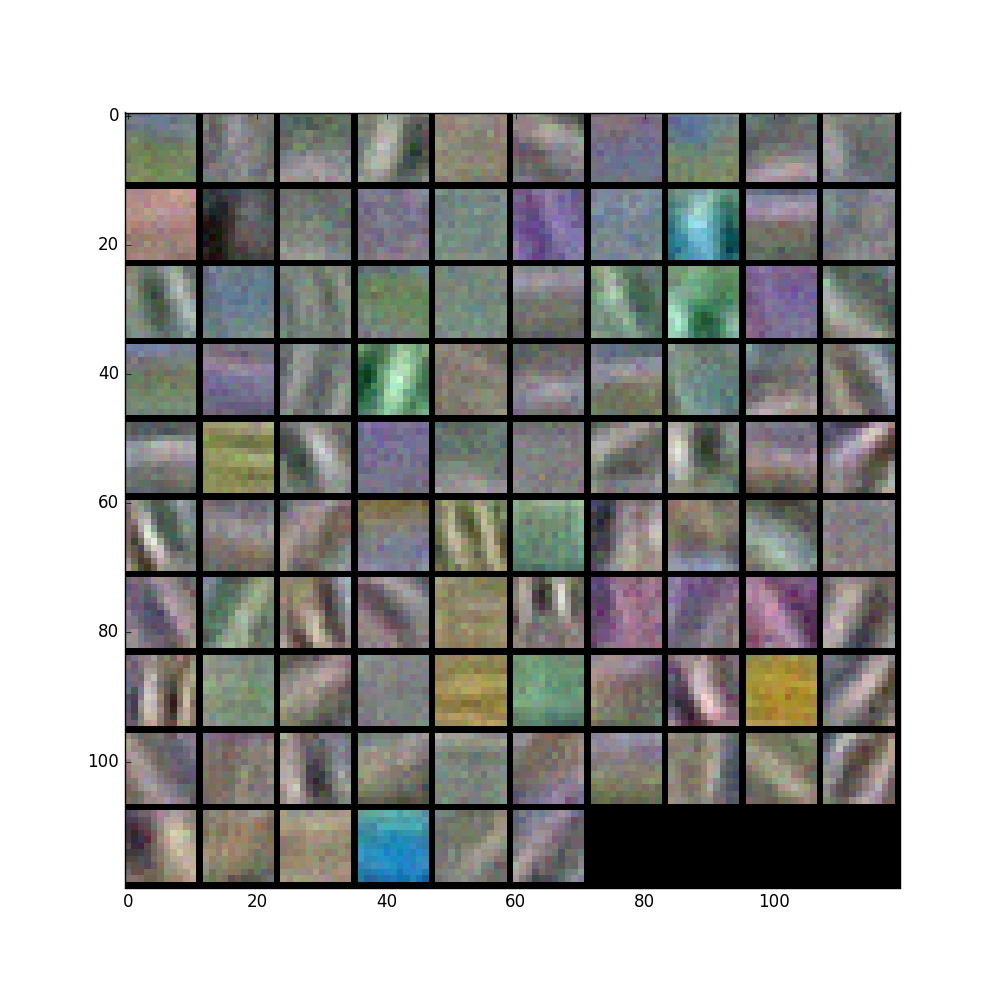
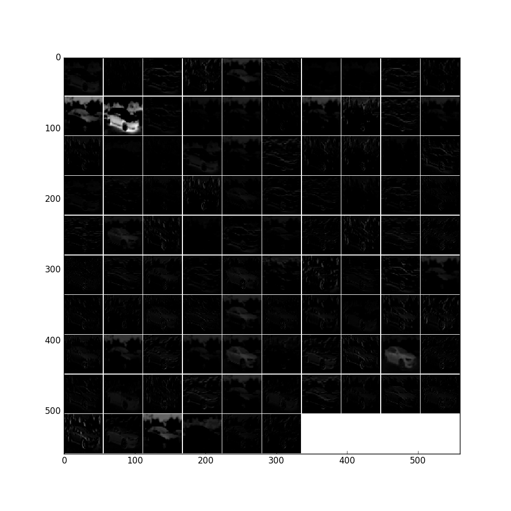
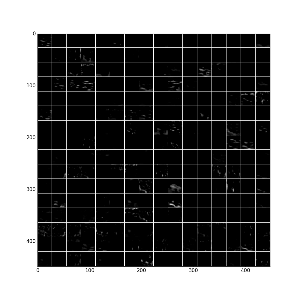
'conv1'输出结果：

feat = net.blobs['conv1'].data[0, :96]

vis_square(feat, padval=1)

 

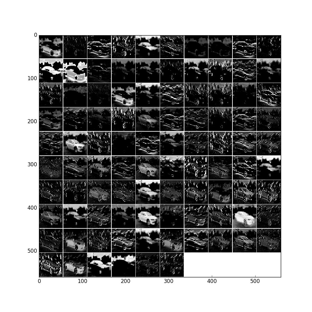
'norm1'输出结果：

 

feat = net.blobs['norm1'].data[0]

vis_square(feat, padval=1)

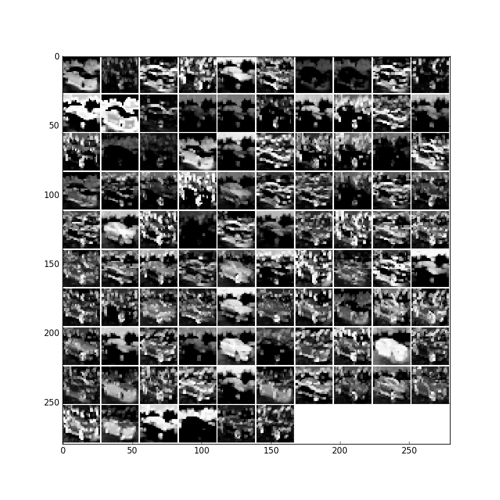
feat = net.blobs['pool1'].data[0]

vis_square(feat, padval=1)

 

 

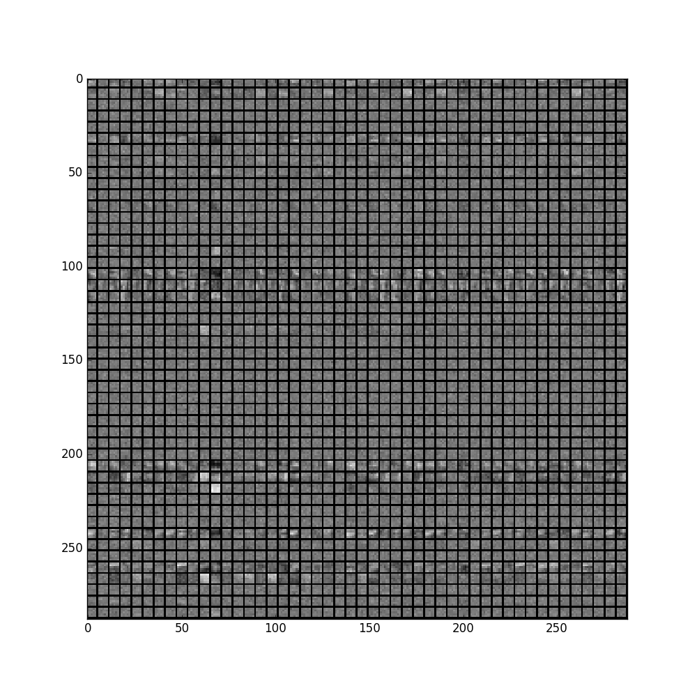
filters = net.params['conv2'][0].data

vis_square(filters[:48].reshape(48**2, 5, 5))

 

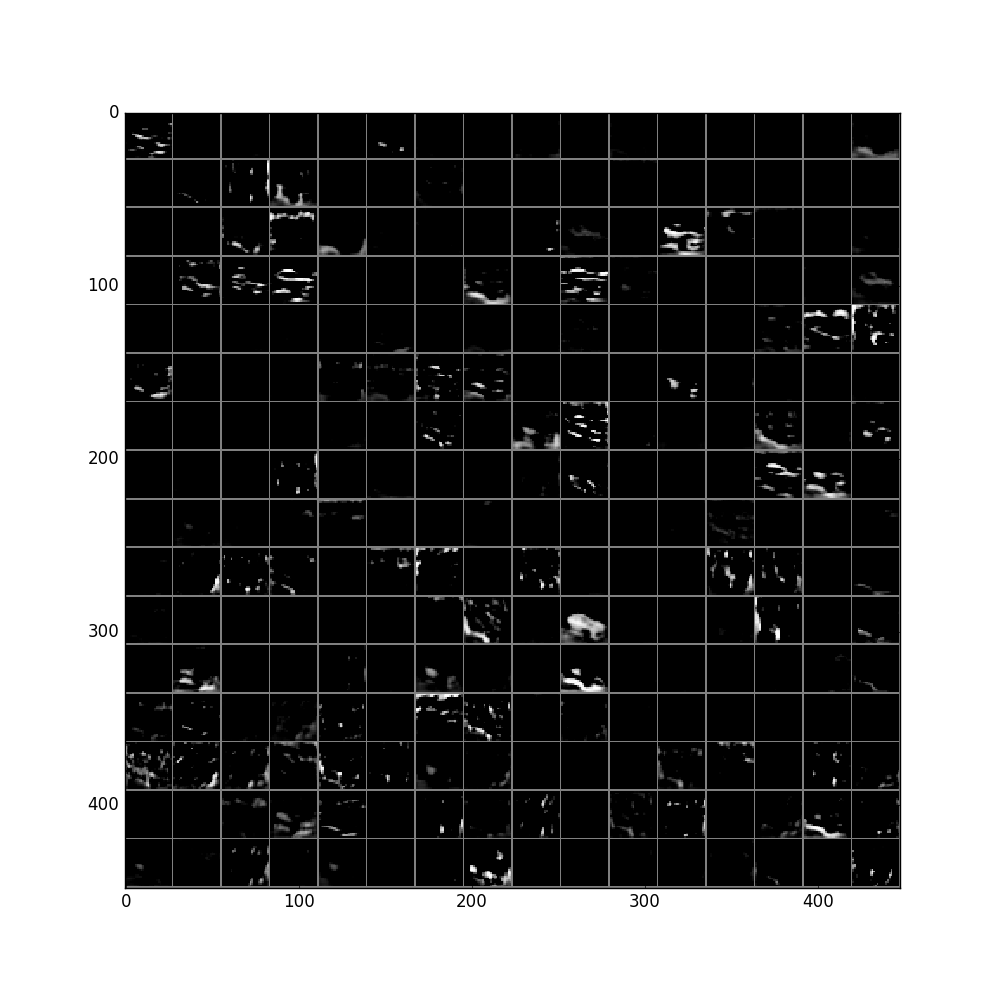
feat = net.blobs['conv2'].data[0]

vis_square(feat, padval=1)

feat = net.blobs['norm2'].data[0]

vis_square(feat, padval=0.5)

 

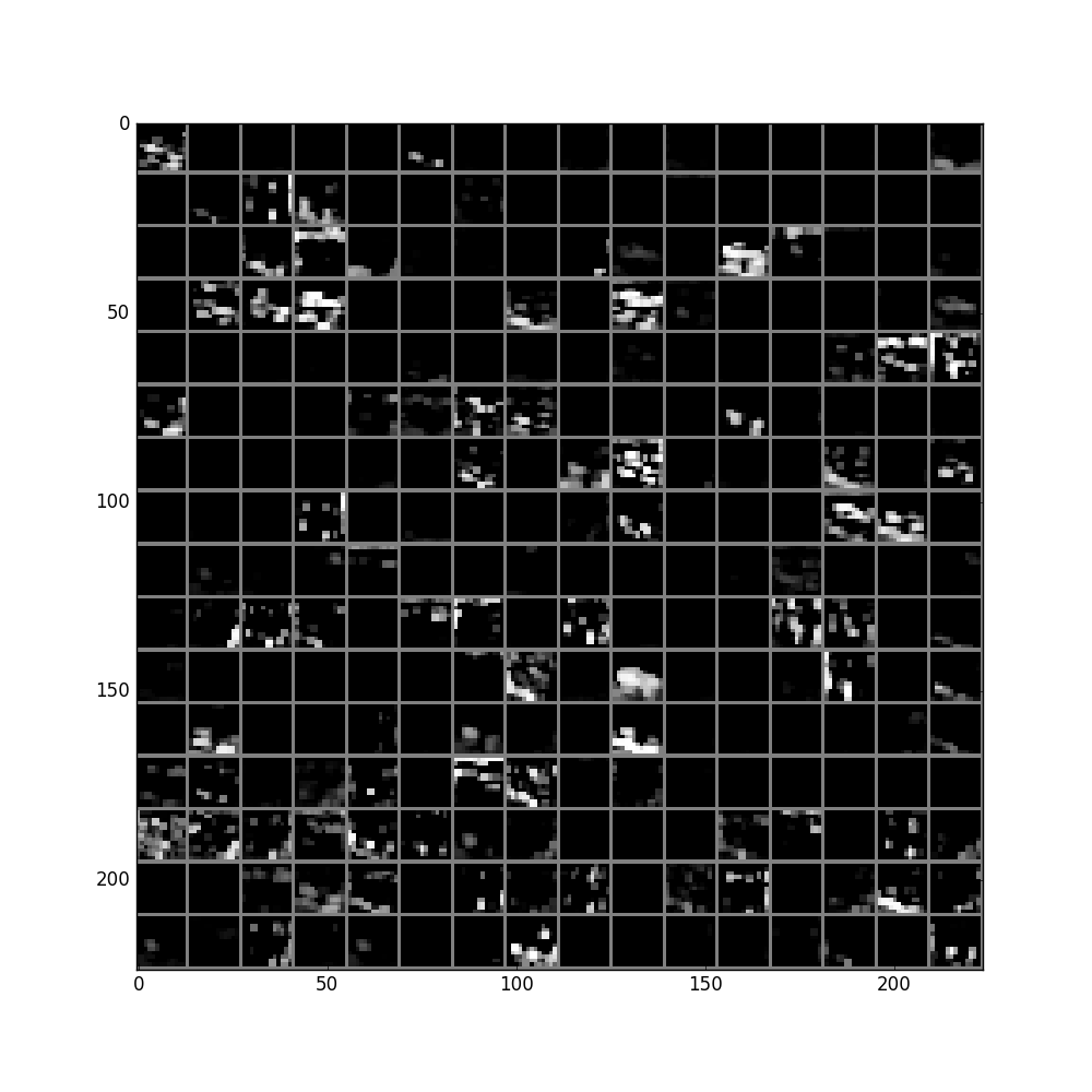
feat = net.blobs['pool2'].data[0]

vis_square(feat, padval=0.5)

可以看出越到高层越抽象，pool层信息损失很大。

中间省略n层。。。

pool5层：

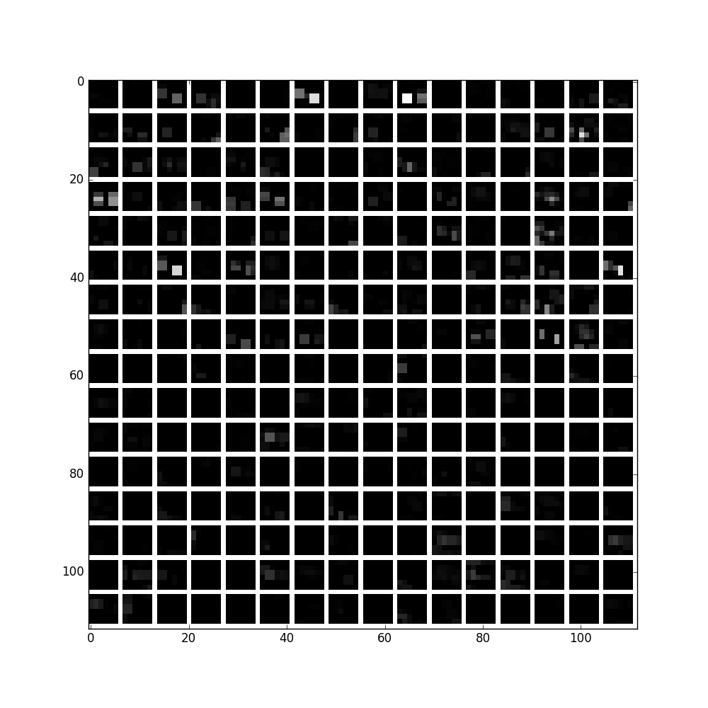
fc6及其直方图：

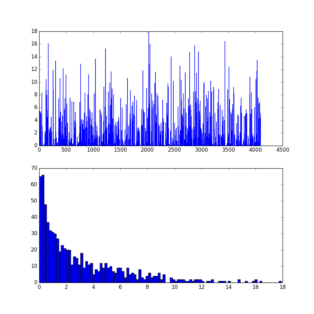
 。。。只能说太奇妙太强大，就是这样莫名其妙的net就能高准确率的辨别出来车子了！

部分代码：

import numpy as np
import matplotlib.pyplot as plt




# Make sure that caffe is on the python path:
caffe_root = 'E:/machinelearning/code/caffe-windows/'  # this file is expected to be in {caffe_root}/examples
import sys
sys.path.insert(0, caffe_root + 'python')


import caffe


plt.rcParams['figure.figsize'] = (10,10)
plt.rcParams['image.interpolation'] = 'nearest'
plt.rcParams['image.cmap'] = 'gray'


import os
if not os.path.isfile(caffe_root + 'models/bvlc_reference_caffenet/bvlc_reference_caffenet.caffemodel'):
    print("Downloading pre-trained CaffeNet model...")
caffe.set_mode_cpu()
net = caffe.Net(caffe_root + 'models/bvlc_reference_caffenet/deploy.prototxt',
                caffe_root + 'models/bvlc_reference_caffenet/bvlc_reference_caffenet.caffemodel',
                caffe.TEST)


# input preprocessing: 'data' is the name of the input blob == net.inputs[0]
transformer = caffe.io.Transformer({'data': net.blobs['data'].data.shape})
transformer.set_transpose('data', (2,0,1))
transformer.set_mean('data', np.load(caffe_root + 'python/caffe/imagenet/ilsvrc_2012_mean.npy').mean(1).mean(1)) # mean pixel
transformer.set_raw_scale('data', 255)  # the reference model operates on images in [0,255] range instead of [0,1]
transformer.set_channel_swap('data', (2,1,0))  # the reference model has channels in BGR order instead of RGB
net.blobs['data'].reshape(50,3,227,227)
net.blobs['data'].data[...] = transformer.preprocess('data', caffe.io.load_image(caffe_root + 'examples/images/cat.jpg'))
out = net.forward()
print("Predicted clss is #{}.".format(out['prob'][0].argmax()))
plt.imshow(transformer.deprocess('data', net.blobs['data'].data[0]))
# load labels
imagenet_labels_filename = caffe_root + 'examples/GoogLeNet/synset_words.txt'
try:
    labels = np.loadtxt(imagenet_labels_filename, str, delimiter='\t')
except:
    labels = np.loadtxt(imagenet_labels_filename, str, delimiter='\t')


# sort top k predictions from softmax output
top_k = net.blobs['prob'].data[0].flatten().argsort()[-1:-6:-1]
print labels[top_k]


def vis_square(data, padsize=1, padval=0):
    data -= data.min()
    data /= data.max()
    
    # force the number of filters to be square
    n = int(np.ceil(np.sqrt(data.shape[0])))
    padding = ((0, n ** 2 - data.shape[0]), (0, padsize), (0, padsize)) + ((0, 0),) * (data.ndim - 3)
    data = np.pad(data, padding, mode='constant', constant_values=(padval, padval))
    
    # tile the filters into an image
    data = data.reshape((n, n) + data.shape[1:]).transpose((0, 2, 1, 3) + tuple(range(4, data.ndim + 1)))
    data = data.reshape((n * data.shape[1], n * data.shape[3]) + data.shape[4:])
    
    plt.imshow(data)
# the parameters are a list of [weights, biases]
filters = net.params['conv1'][0].data
vis_square(filters.transpose(0, 2, 3, 1))
plt.show()

参考文件：http://nbviewer.ipython.org/github/BVLC/caffe/blob/master/examples/00-classification.ipynb