《利用python做数据分析》第十章：时间序列分析

最新推荐文章于 2024-05-14 09:07:31 发布

wx1871428

最新推荐文章于 2024-05-14 09:07:31 发布

阅读量181

点赞数

分类专栏： Python 时间序列

本文链接：https://blog.csdn.net/wx1871428/article/details/118328495

版权

Python 同时被 2 个专栏收录

156 篇文章 12 订阅

订阅专栏

时间序列

2 篇文章 0 订阅

订阅专栏

    import pandas as pd
    import numpy as np
    import matplotlib.pyplot as plt
    %matplotlib inline
[/code]

//anaconda/lib/python2.7/site-packages/matplotlib/font_manager.py:273:
UserWarning: Matplotlib is building the font cache using fc-list. This may
take a moment. warnings.warn(‘Matplotlib is building the font cache using fc-
list. This may take a moment.’)

```code
    from pandas import Series,DataFrame
[/code]

#### Time Seiries Analysis **** > build-in package time datetime calendar

```code
    from datetime import datetime
[/code]

```code
    now = datetime.now()
[/code]

```code
    now
[/code]

datetime.datetime(2016, 2, 1, 11, 11, 8, 934671) > ** display time right now
**

```code
    now.year,now.month,now.day
[/code]

(2016, 2, 1) datetime以毫秒形势存储��和⌚️，**datetime.datedelta**表示两个datetime对象之间的时间差

```code
    delta = datetime(2011,1,7) - datetime(2008,6,24,8,15)
[/code]

显示的前一个是天数，后一个是秒钟 —- delta.days delta.seconds

```code
    delta
[/code]

datetime.timedelta(926, 56700) ### 可以给datetime对象加上或者减去一个或者多个timedelta，会产生一个新对象

```code
    from datetime import timedelta
[/code]

```code
    start = datetime(2011, 1, 7)
[/code]

```code
    start + timedelta(12)
[/code]

datetime.datetime(2011, 1, 19, 0, 0)

```code
    start - timedelta(12) * 4
[/code]

datetime.datetime(2010, 11, 20, 0, 0) > 可见timedelta是以天为单位 ####
datetime模块中的数据类型 —– - date | 以公历形式存储日历日期（年、月、日） - time | 将时间存储为时、分、秒、毫秒 -
datetime | 存储时间和日期 - timedelta| 比阿诗两个datetime值之间的差（日， 秒， 毫秒） ## str
transformed to datetime use ** str ** or ** strftime(invoke a formed str) **
,datetime object and pandas.Timestamp can be formulated to string

```code
    stamp = datetime(2011, 1, 3)
[/code]

```code
    str(stamp)
[/code]

‘2011-01-03 00:00:00’

```code
    stamp.strftime('%Y-%m-%d')
[/code]

‘2011-01-03’

```code
    stamp.strftime('%Y-%m')
[/code]

‘2011-01’

```code
    value = '2011-01-03'
[/code]

```code
    datetime.strptime(value, '%Y-%m-%d')
[/code]

datetime.datetime(2011, 1, 3, 0, 0)

```code
    datestrs = ['7/6/2011','8/6/2011']
[/code]

```code
    [datetime.strptime(x, '%m/%d/%Y') for x in datestrs]
[/code]

[datetime.datetime(2011, 7, 6, 0, 0), datetime.datetime(2011, 8, 6, 0, 0)]
datetime.striptime 是通过已知格式进行日期解析的最佳方式，但每次都要编写格式定义 -
使用dateutil中的parser.parse来实现

```code
    from dateutil.parser import parse
[/code]

```code
    parse('2011-01-03')
[/code]

datetime.datetime(2011, 1, 3, 0, 0) parse的解析能力很强，几乎可以解析一切格式

```code
    parse('Jan 31,1997 10:45 PM')
[/code]

datetime.datetime(1997, 1, 31, 22, 45)

```code
    parse('6/30/2011', dayfirst=True)
[/code]

datetime.datetime(2011, 6, 30, 0, 0)

```code
    datestrs
[/code]

[‘7/6/2011’, ‘8/6/2011’] # pd.to_datetime()

```code
    pd.to_datetime(datestrs)
[/code]

DatetimeIndex([‘2011-07-06’, ‘2011-08-06’], dtype=’datetime64[ns]’, freq=None)

```code
    dates = [datetime(2011, 1, 2),datetime(2011,1,5),datetime(2011,1,7),
            datetime(2011,1,8),datetime(2011,1,10),datetime(2011,1,12)]
[/code]

```code
    ts = Series(np.random.randn(6), index=dates)
[/code]

```code
    ts
[/code]

2011-01-02 0.573974 2011-01-05 -0.337112 2011-01-07 -1.650845 2011-01-08
0.450012 2011-01-10 -1.253801 2011-01-12 -0.402997 dtype: float64

```code
    type(ts)
[/code]

pandas.core.series.Series

```code
    ts.index
[/code]

DatetimeIndex([‘2011-01-02’, ‘2011-01-05’, ‘2011-01-07’, ‘2011-01-08’,
‘2011-01-10’, ‘2011-01-12’], dtype=’datetime64[ns]’, freq=None)

```code
    ts + ts[::2]
[/code]

2011-01-02 1.147949 2011-01-05 NaN 2011-01-07 -3.301690 2011-01-08 NaN
2011-01-10 -2.507602 2011-01-12 NaN dtype: float64

```code
    ts[::2]
[/code]

2011-01-02 0.573974 2011-01-07 -1.650845 2011-01-10 -1.253801 dtype: float64
## 索引、选取、子集构造

```code
    ts['1/10/2011']
[/code]

-1.2538008746706757 传入可以解释为日期的字符，就可以代替索引 
```code
    ts['20110110']
[/code]

-1.2538008746706757 
```code
    longer_ts=Series(np.random.randn(1000),index=pd.date_range('20000101',periods=1000))
[/code]

```code
    longer_ts
[/code]

2000-01-01 -1.025498 2000-01-02 -0.913267 2000-01-03 0.240895 2000-01-04
-1.475368 2000-01-05 -1.675558 2000-01-06 1.020005 2000-01-07 0.638097
2000-01-08 0.503482 2000-01-09 -0.541771 2000-01-10 -1.107036 2000-01-11
0.797612 2000-01-12 1.691745 2000-01-13 1.889323 2000-01-14 -0.852126
2000-01-15 -0.987578 2000-01-16 0.558084 2000-01-17 -0.842907 2000-01-18
1.932399 2000-01-19 -1.126650 2000-01-20 -0.529707 2000-01-21 0.116756
2000-01-22 -0.012790 2000-01-23 0.501330 2000-01-24 0.346976 2000-01-25
-0.880443 2000-01-26 -0.229017 2000-01-27 0.926648 2000-01-28 0.894491
2000-01-29 -0.573260 2000-01-30 -1.712945 … 2002-08-28 -0.751376 2002-08-29
-1.731035 2002-08-30 -0.150107 2002-08-31 -0.621332 2002-09-01 0.449311
2002-09-02 0.873422 2002-09-03 1.496143 2002-09-04 -0.581023 2002-09-05
2.882920 2002-09-06 -0.347482 2002-09-07 0.165490 2002-09-08 -0.475642
2002-09-09 0.191958 2002-09-10 0.801963 2002-09-11 -1.603021 2002-09-12
1.114401 2002-09-13 0.994800 2002-09-14 -0.974208 2002-09-15 2.096747
2002-09-16 -0.252620 2002-09-17 -0.279536 2002-09-18 -0.059076 2002-09-19
-0.497615 2002-09-20 -0.009895 2002-09-21 1.813504 2002-09-22 0.863885
2002-09-23 1.330777 2002-09-24 -0.394473 2002-09-25 -1.163973 2002-09-26
-0.986664 Freq: D, dtype: float64

```code
    longer_ts['2002']
[/code]

2002-01-01 -1.249172 2002-01-02 -1.368829 2002-01-03 0.097135 2002-01-04
-0.972259 2002-01-05 -0.640629 2002-01-06 0.619072 2002-01-07 1.625769
2002-01-08 -0.893140 2002-01-09 0.113725 2002-01-10 0.446898 2002-01-11
-0.382041 2002-01-12 -1.667311 2002-01-13 -0.307464 2002-01-14 0.623383
2002-01-15 -0.211188 2002-01-16 -1.166355 2002-01-17 0.399710 2002-01-18
-0.171451 2002-01-19 -1.591578 2002-01-20 -0.367654 2002-01-21 0.985778
2002-01-22 0.125848 2002-01-23 1.366708 2002-01-24 0.449383 2002-01-25
0.211848 2002-01-26 -1.033201 2002-01-27 0.668416 2002-01-28 0.402693
2002-01-29 -0.730690 2002-01-30 1.666659 … 2002-08-28 -0.751376 2002-08-29
-1.731035 2002-08-30 -0.150107 2002-08-31 -0.621332 2002-09-01 0.449311
2002-09-02 0.873422 2002-09-03 1.496143 2002-09-04 -0.581023 2002-09-05
2.882920 2002-09-06 -0.347482 2002-09-07 0.165490 2002-09-08 -0.475642
2002-09-09 0.191958 2002-09-10 0.801963 2002-09-11 -1.603021 2002-09-12
1.114401 2002-09-13 0.994800 2002-09-14 -0.974208 2002-09-15 2.096747
2002-09-16 -0.252620 2002-09-17 -0.279536 2002-09-18 -0.059076 2002-09-19
-0.497615 2002-09-20 -0.009895 2002-09-21 1.813504 2002-09-22 0.863885
2002-09-23 1.330777 2002-09-24 -0.394473 2002-09-25 -1.163973 2002-09-26
-0.986664 Freq: D, dtype: float64

```code
    longer_ts['2001/03']
[/code]

2001-03-01 -0.130463 2001-03-02 -1.245341 2001-03-03 1.035173 2001-03-04
1.115275 2001-03-05 0.013602 2001-03-06 0.828075 2001-03-07 -0.802564
2001-03-08 2.067711 2001-03-09 2.158392 2001-03-10 1.348256 2001-03-11
1.282607 2001-03-12 -1.088485 2001-03-13 -0.882978 2001-03-14 -0.030872
2001-03-15 0.840561 2001-03-16 -0.061428 2001-03-17 0.170721 2001-03-18
0.895892 2001-03-19 -0.050714 2001-03-20 0.608656 2001-03-21 1.222177
2001-03-22 0.889833 2001-03-23 -0.932351 2001-03-24 0.163275 2001-03-25
0.001171 2001-03-26 0.969950 2001-03-27 -0.118747 2001-03-28 -0.840478
2001-03-29 -2.654215 2001-03-30 -0.351836 2001-03-31 -0.365322 Freq: D, dtype:
float64

```code
    ts['20110101':'20110201']
[/code]

2011-01-02 0.573974 2011-01-05 -0.337112 2011-01-07 -1.650845 2011-01-08
0.450012 2011-01-10 -1.253801 2011-01-12 -0.402997 dtype: float64

```code
    ts.truncate(after='20110109')
[/code]

2011-01-02 0.573974 2011-01-05 -0.337112 2011-01-07 -1.650845 2011-01-08
0.450012 dtype: float64

```code
    dates = pd.date_range('20000101', periods=100, freq='W-WED')
[/code]

```code
    dates
[/code]

DatetimeIndex([‘2000-01-05’, ‘2000-01-12’, ‘2000-01-19’, ‘2000-01-26’,
‘2000-02-02’, ‘2000-02-09’, ‘2000-02-16’, ‘2000-02-23’, ‘2000-03-01’,
‘2000-03-08’, ‘2000-03-15’, ‘2000-03-22’, ‘2000-03-29’, ‘2000-04-05’,
‘2000-04-12’, ‘2000-04-19’, ‘2000-04-26’, ‘2000-05-03’, ‘2000-05-10’,
‘2000-05-17’, ‘2000-05-24’, ‘2000-05-31’, ‘2000-06-07’, ‘2000-06-14’,
‘2000-06-21’, ‘2000-06-28’, ‘2000-07-05’, ‘2000-07-12’, ‘2000-07-19’,
‘2000-07-26’, ‘2000-08-02’, ‘2000-08-09’, ‘2000-08-16’, ‘2000-08-23’,
‘2000-08-30’, ‘2000-09-06’, ‘2000-09-13’, ‘2000-09-20’, ‘2000-09-27’,
‘2000-10-04’, ‘2000-10-11’, ‘2000-10-18’, ‘2000-10-25’, ‘2000-11-01’,
‘2000-11-08’, ‘2000-11-15’, ‘2000-11-22’, ‘2000-11-29’, ‘2000-12-06’,
‘2000-12-13’, ‘2000-12-20’, ‘2000-12-27’, ‘2001-01-03’, ‘2001-01-10’,
‘2001-01-17’, ‘2001-01-24’, ‘2001-01-31’, ‘2001-02-07’, ‘2001-02-14’,
‘2001-02-21’, ‘2001-02-28’, ‘2001-03-07’, ‘2001-03-14’, ‘2001-03-21’,
‘2001-03-28’, ‘2001-04-04’, ‘2001-04-11’, ‘2001-04-18’, ‘2001-04-25’,
‘2001-05-02’, ‘2001-05-09’, ‘2001-05-16’, ‘2001-05-23’, ‘2001-05-30’,
‘2001-06-06’, ‘2001-06-13’, ‘2001-06-20’, ‘2001-06-27’, ‘2001-07-04’,
‘2001-07-11’, ‘2001-07-18’, ‘2001-07-25’, ‘2001-08-01’, ‘2001-08-08’,
‘2001-08-15’, ‘2001-08-22’, ‘2001-08-29’, ‘2001-09-05’, ‘2001-09-12’,
‘2001-09-19’, ‘2001-09-26’, ‘2001-10-03’, ‘2001-10-10’, ‘2001-10-17’,
‘2001-10-24’, ‘2001-10-31’, ‘2001-11-07’, ‘2001-11-14’, ‘2001-11-21’,
‘2001-11-28’], dtype=’datetime64[ns]’, freq=’W-WED’)

```code
    long_df = DataFrame(np.random.randn(100,4),index=dates,columns=['Colorado','Texas','New York','Ohio'])
[/code]

```code
    long_df.ix['5-2001']
[/code]

|  Colorado  |  Texas  |  New York  |  Ohio  
---|---|---|---|---  
2001-05-02  |  1.783070  |  1.090816  |  -1.035363  |  -0.089864  
2001-05-09  |  -1.290700  |  1.311863  |  -0.596037  |  0.819694  
2001-05-16  |  0.688693  |  -0.249644  |  -0.859212  |  0.879270  
2001-05-23  |  -1.602660  |  1.211236  |  -1.028336  |  2.022514  
2001-05-30  |  -0.705427  |  -0.189235  |  -0.710712  |  -2.397815

```code
    dates = pd.DatetimeIndex(['1/1/2000','1/2/2000',
                             '1/2/2000','1/2/2000',
                             '1/3/2000'])
[/code]

```code
    dup_ts = Series(np.arange(5), index=dates)
[/code]

```code
    dup_ts
[/code]  
  
2000-01-01 0 2000-01-02 1 2000-01-02 2 2000-01-02 3 2000-01-03 4 dtype: int64
通过检查索引的** is_unique ** 属性，判断是不是唯一

```code
    dup_ts.index.is_unique
[/code]

False 对这个时间序列进行索引，要么产生标量值，要么产生切片，具体要看所选的 > **时间点是否重复** none repeat(2000-1-3)

```code
    dup_ts['1/3/2000']
[/code]

4 repeat (2000-1-2)

```code
    dup_ts['1/2/2000']
[/code]

2000-01-02 1 2000-01-02 2 2000-01-02 3 dtype: int64 define whether it is
reaptable or not

```code
    dup_ts.index.is_unique
[/code]

False # 对具有非唯一时间戳的数据聚合 # > groupby(level=0) level=0意味着索引唯一一层！！！ —-

```code
    grouped = dup_ts.groupby(level=0)
[/code]

```code
    grouped.mean(),grouped.count()
[/code]

(2000-01-01 0 2000-01-02 2 2000-01-03 4 dtype: int64, 2000-01-01 1 2000-01-02
3 2000-01-03 1 dtype: int64) > 将时间序列转换成 **具有固定频率（每日）的时间序列** - resample

```code
    ts.resample('D')
[/code]

2011-01-02 0.573974 2011-01-03 NaN 2011-01-04 NaN 2011-01-05 -0.337112
2011-01-06 NaN 2011-01-07 -1.650845 2011-01-08 0.450012 2011-01-09 NaN
2011-01-10 -1.253801 2011-01-11 NaN 2011-01-12 -0.402997 Freq: D, dtype:
float64 生成日期范围 - pandas.date_range - 类型：DatetimeIndex

```code
    index = pd.date_range('4/1/2012','6/1/2012')
[/code]

## base frequency - 基础频率通常以一个字符串表示，M每月，H每小时 - 对于每个基础频率都有一个偏移量与之对应 - date
offset

```code
    from pandas.tseries.offsets import Hour, Minute
[/code]

```code
    hour = Hour()
[/code]

```code
    hour
[/code]

> 传入一个整数即可定义偏移量的倍数：
```code
    four_hours = Hour(4)
[/code]

```code
    four_hours
[/code]

```code
    pd.date_range('1/1/2000','1/3/2000 23:59',freq='4h')
[/code]

DatetimeIndex([‘2000-01-01 00:00:00’, ‘2000-01-01 04:00:00’, ‘2000-01-01
08:00:00’, ‘2000-01-01 12:00:00’, ‘2000-01-01 16:00:00’, ‘2000-01-01
20:00:00’, ‘2000-01-02 00:00:00’, ‘2000-01-02 04:00:00’, ‘2000-01-02
08:00:00’, ‘2000-01-02 12:00:00’, ‘2000-01-02 16:00:00’, ‘2000-01-02
20:00:00’, ‘2000-01-03 00:00:00’, ‘2000-01-03 04:00:00’, ‘2000-01-03
08:00:00’, ‘2000-01-03 12:00:00’, ‘2000-01-03 16:00:00’, ‘2000-01-03
20:00:00’], dtype=’datetime64[ns]’, freq=’4H’) 偏移量可以通过加法链接

```code
    Hour(2) + Minute(30)
[/code]

```code
    pd.date_range('1/1/2000', periods=10, freq='1h30min')
[/code]

DatetimeIndex([‘2000-01-01 00:00:00’, ‘2000-01-01 01:30:00’, ‘2000-01-01
03:00:00’, ‘2000-01-01 04:30:00’, ‘2000-01-01 06:00:00’, ‘2000-01-01
07:30:00’, ‘2000-01-01 09:00:00’, ‘2000-01-01 10:30:00’, ‘2000-01-01
12:00:00’, ‘2000-01-01 13:30:00’], dtype=’datetime64[ns]’, freq=’90T’) ###
WOM(week of month)

```code
    rng = pd.date_range('1/1/2012','9/1/2012',freq='WOM-3FRI')
[/code]

```code
    pd.date_range('1/1/2012','9/1/2012',freq='W-FRI')
[/code]

DatetimeIndex([‘2012-01-06’, ‘2012-01-13’, ‘2012-01-20’, ‘2012-01-27’,
‘2012-02-03’, ‘2012-02-10’, ‘2012-02-17’, ‘2012-02-24’, ‘2012-03-02’,
‘2012-03-09’, ‘2012-03-16’, ‘2012-03-23’, ‘2012-03-30’, ‘2012-04-06’,
‘2012-04-13’, ‘2012-04-20’, ‘2012-04-27’, ‘2012-05-04’, ‘2012-05-11’,
‘2012-05-18’, ‘2012-05-25’, ‘2012-06-01’, ‘2012-06-08’, ‘2012-06-15’,
‘2012-06-22’, ‘2012-06-29’, ‘2012-07-06’, ‘2012-07-13’, ‘2012-07-20’,
‘2012-07-27’, ‘2012-08-03’, ‘2012-08-10’, ‘2012-08-17’, ‘2012-08-24’,
‘2012-08-31’], dtype=’datetime64[ns]’, freq=’W-FRI’) > 时间表别名10-4 P314 ###
移动（超前和滞后）数据 - 移动（shifting）指的是沿着时间轴将数据迁移或者后移 - Series &
Dataframe都有一个shift方法单纯执行前移后移 - 保持索引不变

```code
    ts = Series(np.random.randn(4),index=pd.date_range('1/1/2000',periods=4,freq='M'))
[/code]

```code
    ts
[/code]

2000-01-31 -0.550830 2000-02-29 -1.297499 2000-03-31 1.178102 2000-04-30
1.359573 Freq: M, dtype: float64

```code
    ts.shift(-2)
[/code]

2000-01-31 1.178102 2000-02-29 1.359573 2000-03-31 NaN 2000-04-30 NaN Freq: M,
dtype: float64 shift ususally used to calculate the pct change of a series

```code
    ts / ts.shift(1) - 1
[/code]

2000-01-31 NaN 2000-02-29 1.355534 2000-03-31 -1.907979 2000-04-30 0.154037
Freq: M, dtype: float64

```code
    ts.pct_change()
[/code]

2000-01-31 NaN 2000-02-29 1.355534 2000-03-31 -1.907979 2000-04-30 0.154037
Freq: M, dtype: float64

```code
    ts.shift(2, freq='M')
[/code]

2000-03-31 -0.550830 2000-04-30 -1.297499 2000-05-31 1.178102 2000-06-30
1.359573 Freq: M, dtype: float64

```code
    ts.shift(3, freq='D')
[/code]

2000-02-03 -0.550830 2000-03-03 -1.297499 2000-04-03 1.178102 2000-05-03
1.359573 dtype: float64

```code
    type(ts)
[/code]

pandas.core.series.Series

```code
    ts.shift()
[/code]

2000-01-31 NaN 2000-02-29 -0.550830 2000-03-31 -1.297499 2000-04-30 1.178102
Freq: M, dtype: float64

```code
    ts.shift(3)
[/code]

2000-01-31 NaN 2000-02-29 NaN 2000-03-31 NaN 2000-04-30 -0.55083 Freq: M,
dtype: float64

```code
    ts.shift(freq='D')
[/code]

2000-02-01 -0.550830 2000-03-01 -1.297499 2000-04-01 1.178102 2000-05-01
1.359573 Freq: MS, dtype: float64

```code
    ts.shift(periods=2)
[/code]

2000-01-31 NaN 2000-02-29 NaN 2000-03-31 -0.550830 2000-04-30 -1.297499 Freq:
M, dtype: float64 freq means move the index by the frequence

```code
    from pandas.tseries.offsets import Day, MonthEnd
[/code]

如果增加的是⚓️点偏移量（比如MonthEnd)，第一次增量会讲原来的日期向前滚动到适合规则的下一个日期 -
今天11月17号，MonthEnd就是这个月末11.31

```code
    now = datetime(2011, 11, 17)
[/code]

```code
    now + 3*Day()
[/code]

Timestamp(‘2011-11-20 00:00:00’)

```code
    now + MonthEnd()
[/code]

Timestamp(‘2011-11-30 00:00:00’)

```code
    now + MonthEnd(2)
[/code]

Timestamp(‘2011-12-31 00:00:00’)

```code
    offset = MonthEnd()
[/code]

```code
    offset.rollforward(now)
[/code]

Timestamp(‘2011-11-30 00:00:00’)

```code
    offset.rollback(now)
[/code]

Timestamp(‘2011-10-31 00:00:00’) 巧妙的使用**groupby**和**⚓️点偏移量**

```code
    ts = Series(np.random.randn(20), index=pd.date_range('1/15/2000',periods=20,freq='4d'))
[/code]

```code
    ts.groupby(offset.rollforward).mean()
[/code]

2000-01-31 -0.223943 2000-02-29 -0.241283 2000-03-31 -0.080391 dtype: float64
更方便快捷的方法应该是用 > resample

```code
    ts.resample('M', how='mean')
[/code]

2000-01-31 -0.223943 2000-02-29 -0.241283 2000-03-31 -0.080391 Freq: M, dtype:
float64 # import pytz —- pytz是一个世界时区的库，时区名

```code
    import pytz
[/code]

```code
    pytz.common_timezones[-5:]
[/code]

[‘US/Eastern’, ‘US/Hawaii’, ‘US/Mountain’, ‘US/Pacific’, ‘UTC’]

```code
    tz = pytz.timezone('US/Eastern')
[/code]

```code
    tz
[/code]

### 本地化和转换

```code
    rng = pd.date_range('3/9/2012 9:30',periods=6, freq='D')
    ts = Series(np.random.randn(len(rng)),index=rng)
[/code]

```code
    del index
[/code]

```code
    ts.index.tz
[/code]

add a time zone set of the ts - make it print

```code
    pd.date_range('3/9/2000 9:30',periods=10, freq='D',tz='UTC')
[/code]

DatetimeIndex([‘2000-03-09 09:30:00+00:00’, ‘2000-03-10 09:30:00+00:00’,
‘2000-03-11 09:30:00+00:00’, ‘2000-03-12 09:30:00+00:00’, ‘2000-03-13
09:30:00+00:00’, ‘2000-03-14 09:30:00+00:00’, ‘2000-03-15 09:30:00+00:00’,
‘2000-03-16 09:30:00+00:00’, ‘2000-03-17 09:30:00+00:00’, ‘2000-03-18
09:30:00+00:00’], dtype=’datetime64[ns, UTC]’, freq=’D’) > The +00:00 means -
time zone use *tz_localize* to localize the time zone

```code
    ts_utc = ts.tz_localize('UTC')
    
    ts_utc
[/code]

2012-03-09 09:30:00+00:00 -0.258702 2012-03-10 09:30:00+00:00 -1.019056
2012-03-11 09:30:00+00:00 1.044139 2012-03-12 09:30:00+00:00 0.826684
2012-03-13 09:30:00+00:00 0.998759 2012-03-14 09:30:00+00:00 -0.839695 Freq:
D, dtype: float64 just have a try of crtl+v

```code
    ts_utc.index
[/code]

DatetimeIndex([‘2012-03-09 09:30:00+00:00’, ‘2012-03-10 09:30:00+00:00’,
‘2012-03-11 09:30:00+00:00’, ‘2012-03-12 09:30:00+00:00’, ‘2012-03-13
09:30:00+00:00’, ‘2012-03-14 09:30:00+00:00’], dtype=’datetime64[ns, UTC]’,
freq=’D’) convert localized time zone to another one use: > *tz_convert*

```code
    ts_utc.tz_convert('US/Eastern')
[/code]

2012-03-09 04:30:00-05:00 -0.258702 2012-03-10 04:30:00-05:00 -1.019056
2012-03-11 05:30:00-04:00 1.044139 2012-03-12 05:30:00-04:00 0.826684
2012-03-13 05:30:00-04:00 0.998759 2012-03-14 05:30:00-04:00 -0.839695 Freq:
D, dtype: float64 *tz_localize* & *tz_convert* are also instance methods on
*DatetimeIndex*

```code
    ts.index.tz_localize('Asia/Shanghai')
[/code]

DatetimeIndex([‘2012-03-09 09:30:00+08:00’, ‘2012-03-10 09:30:00+08:00’,
‘2012-03-11 09:30:00+08:00’, ‘2012-03-12 09:30:00+08:00’, ‘2012-03-13
09:30:00+08:00’, ‘2012-03-14 09:30:00+08:00’], dtype=’datetime64[ns,
Asia/Shanghai]’, freq=’D’) # operations with Time Zone - awrae Timestamp
Objects Localized from naive to time zone-aware and converted from one time
zone to another

```code
    stamp = pd.Timestamp('2011-03-12 4:00')
    stamp_utc = stamp.tz_localize('utc')
[/code]

```code
    stamp_utc.tz_convert('US/Eastern')
[/code]

Timestamp(‘2011-03-11 23:00:00-0500’, tz=’US/Eastern’) >Time zone-aware
Timestamp objects internally store a UTC timestamp calue as nano-seconed since
thr UNIX epoch(January 1,1970) - this UTC value is invariant between time zone
conversions

```code
    stamp_utc.value
[/code]

1299902400000000000

```code
    stamp = pd.Timestamp('2012-03-12 01:30', tz='US/Eastern')
[/code]

```code
    stamp
[/code]

Timestamp(‘2012-03-12 01:30:00-0400’, tz=’US/Eastern’)

```code
    stamp + Hour()
[/code]

Timestamp(‘2012-03-12 02:30:00-0400’, tz=’US/Eastern’) # operations between
different time zones

```code
    rng = pd.date_range('3/7/2012 9:30',periods=10, freq='B')
[/code]

```code
    ts = Series(np.random.randn(len(rng)), index=rng)
[/code]

```code
    ts
[/code]

2012-03-07 09:30:00 0.315600 2012-03-08 09:30:00 0.616440 2012-03-09 09:30:00
-1.633940 2012-03-12 09:30:00 0.260501 2012-03-13 09:30:00 -0.394620
2012-03-14 09:30:00 -0.554103 2012-03-15 09:30:00 2.441851 2012-03-16 09:30:00
-3.473308 2012-03-19 09:30:00 -0.339365 2012-03-20 09:30:00 0.335510 Freq: B,
dtype: float64

```code
    ts1 = ts[:7].tz_localize('Europe/London')
[/code]

```code
    ts2 = ts1[2:].tz_convert('Europe/Moscow')
[/code]

```code
    result = ts1 + ts2
[/code]

>different time zone can be added up together freely

```code
    result.index
[/code]

DatetimeIndex([‘2012-03-07 09:30:00+00:00’, ‘2012-03-08 09:30:00+00:00’,
‘2012-03-09 09:30:00+00:00’, ‘2012-03-12 09:30:00+00:00’, ‘2012-03-13
09:30:00+00:00’, ‘2012-03-14 09:30:00+00:00’, ‘2012-03-15 09:30:00+00:00’],
dtype=’datetime64[ns, UTC]’, freq=’B’) ## Periods and Periods Arithmetic >
Periods - time spans - days, months,quarters,years

```code
    p = pd.Period(2007, freq='A-DEC')
[/code]

```code
    p
[/code]

Period(‘2007’, ‘A-DEC’) ## Time Series Plotting

```code
    close_px_call = pd.read_csv('/Users/Houbowei/Desktop/SRP/books/pydata-book-master/pydata-book-master/ch09/stock_px.csv', parse_dates=True,index_col=0)
[/code]

```code
    close_px = close_px_call[['AAPL','MSFT','XOM']]
[/code]

```code
    close_px = close_px.resample('B',fill_method='ffill')
[/code]

```code
    close_px
[/code]

|  AAPL  |  MSFT  |  XOM  
---|---|---|---  
2003-01-02  |  7.40  |  21.11  |  29.22  
2003-01-03  |  7.45  |  21.14  |  29.24  
2003-01-06  |  7.45  |  21.52  |  29.96  
2003-01-07  |  7.43  |  21.93  |  28.95  
2003-01-08  |  7.28  |  21.31  |  28.83  
2003-01-09  |  7.34  |  21.93  |  29.44  
2003-01-10  |  7.36  |  21.97  |  29.03  
2003-01-13  |  7.32  |  22.16  |  28.91  
2003-01-14  |  7.30  |  22.39  |  29.17  
2003-01-15  |  7.22  |  22.11  |  28.77  
2003-01-16  |  7.31  |  21.75  |  28.90  
2003-01-17  |  7.05  |  20.22  |  28.60  
2003-01-20  |  7.05  |  20.22  |  28.60  
2003-01-21  |  7.01  |  20.17  |  27.94  
2003-01-22  |  6.94  |  20.04  |  27.58  
2003-01-23  |  7.09  |  20.54  |  27.52  
2003-01-24  |  6.90  |  19.59  |  26.93  
2003-01-27  |  7.07  |  19.32  |  26.21  
2003-01-28  |  7.29  |  19.18  |  26.90  
2003-01-29  |  7.47  |  19.61  |  27.88  
2003-01-30  |  7.16  |  18.95  |  27.37  
2003-01-31  |  7.18  |  18.65  |  28.13  
2003-02-03  |  7.33  |  19.08  |  28.52  
2003-02-04  |  7.30  |  18.59  |  28.52  
2003-02-05  |  7.22  |  18.45  |  28.11  
2003-02-06  |  7.22  |  18.63  |  27.87  
2003-02-07  |  7.07  |  18.30  |  27.66  
2003-02-10  |  7.18  |  18.62  |  27.87  
2003-02-11  |  7.18  |  18.25  |  27.67  
2003-02-12  |  7.20  |  18.25  |  27.12  
…  |  …  |  …  |  …  
2011-09-05  |  374.05  |  25.80  |  72.14  
2011-09-06  |  379.74  |  25.51  |  71.15  
2011-09-07  |  383.93  |  26.00  |  73.65  
2011-09-08  |  384.14  |  26.22  |  72.82  
2011-09-09  |  377.48  |  25.74  |  71.01  
2011-09-12  |  379.94  |  25.89  |  71.84  
2011-09-13  |  384.62  |  26.04  |  71.65  
2011-09-14  |  389.30  |  26.50  |  72.64  
2011-09-15  |  392.96  |  26.99  |  74.01  
2011-09-16  |  400.50  |  27.12  |  74.55  
2011-09-19  |  411.63  |  27.21  |  73.70  
2011-09-20  |  413.45  |  26.98  |  74.01  
2011-09-21  |  412.14  |  25.99  |  71.97  
2011-09-22  |  401.82  |  25.06  |  69.24  
2011-09-23  |  404.30  |  25.06  |  69.31  
2011-09-26  |  403.17  |  25.44  |  71.72  
2011-09-27  |  399.26  |  25.67  |  72.91  
2011-09-28  |  397.01  |  25.58  |  72.07  
2011-09-29  |  390.57  |  25.45  |  73.88  
2011-09-30  |  381.32  |  24.89  |  72.63  
2011-10-03  |  374.60  |  24.53  |  71.15  
2011-10-04  |  372.50  |  25.34  |  72.83  
2011-10-05  |  378.25  |  25.89  |  73.95  
2011-10-06  |  377.37  |  26.34  |  73.89  
2011-10-07  |  369.80  |  26.25  |  73.56  
2011-10-10  |  388.81  |  26.94  |  76.28  
2011-10-11  |  400.29  |  27.00  |  76.27  
2011-10-12  |  402.19  |  26.96  |  77.16  
2011-10-13  |  408.43  |  27.18  |  76.37  
2011-10-14  |  422.00  |  27.27  |  78.11  
  
2292 rows × 3 columns

```code
    close_px.resample?
[/code]

```code
    close_px['AAPL'].plot()
[/code]

```code
    close_px.ix['2009'].plot()
[/code]

```code
    close_px['AAPL'].ix['01-2011':'03-2011'].plot()
[/code]

```code
    apple_q = close_px['AAPL'].resample('Q-DEC', fill_method='ffill')
[/code]

```code
    apple_q.ix['2009':].plot()
[/code]

```code
    close_px.AAPL.plot()
[/code]

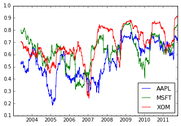
```code
    close_px.plot()
[/code]

```code
    apple_std250 = pd.rolling_std(close_px.AAPL, 250)
[/code]

```code
    apple_std250.describe()
[/code]

count 2043.000000 mean 20.604571 std 12.606813 min 1.335707 25% 9.121461 50%
22.231490 75% 32.411445 max 39.327273 Name: AAPL, dtype: float64

```code
    apple_std250.plot()
[/code]

```code
    close_px.describe()
[/code]

|  AAPL  |  MSFT  |  XOM  
---|---|---|---  
count  |  2292.000000  |  2292.000000  |  2292.000000  
mean  |  125.339895  |  23.953010  |  59.568473  
std  |  107.218553  |  3.267322  |  16.731836  
min  |  6.560000  |  14.330000  |  26.210000  
25%  |  37.122500  |  21.690000  |  49.517500  
50%  |  91.365000  |  24.000000  |  62.980000  
75%  |  185.535000  |  26.280000  |  72.540000  
max  |  422.000000  |  34.070000  |  87.480000

```code
    close_px_call.describe()
[/code]  
  
|  AAPL  |  MSFT  |  XOM  |  SPX  
---|---|---|---|---  
count  |  2214.000000  |  2214.000000  |  2214.000000  |  2214.000000  
mean  |  125.516147  |  23.945452  |  59.558744  |  1183.773311  
std  |  107.394693  |  3.255198  |  16.725025  |  180.983466  
min  |  6.560000  |  14.330000  |  26.210000  |  676.530000  
25%  |  37.135000  |  21.700000  |  49.492500  |  1077.060000  
50%  |  91.455000  |  24.000000  |  62.970000  |  1189.260000  
75%  |  185.605000  |  26.280000  |  72.510000  |  1306.057500  
max  |  422.000000  |  34.070000  |  87.480000  |  1565.150000

```code
    spx = close_px_call.SPX.pct_change()
[/code]

```code
    spx
[/code]

```code
    2003-01-02         NaN
    2003-01-03   -0.000484
    2003-01-06    0.022474
    2003-01-07   -0.006545
    2003-01-08   -0.014086
    2003-01-09    0.019386
    2003-01-10    0.000000
    2003-01-13   -0.001412
    2003-01-14    0.005830
    2003-01-15   -0.014426
    2003-01-16   -0.003942
    2003-01-17   -0.014017
    2003-01-21   -0.015702
    2003-01-22   -0.010432
    2003-01-23    0.010224
    2003-01-24   -0.029233
    2003-01-27   -0.016160
    2003-01-28    0.013050
    2003-01-29    0.006779
    2003-01-30   -0.022849
    2003-01-31    0.013130
    2003-02-03    0.005399
    2003-02-04   -0.014088
    2003-02-05   -0.005435
    2003-02-06   -0.006449
    2003-02-07   -0.010094
    2003-02-10    0.007569
    2003-02-11   -0.008098
    2003-02-12   -0.012687
    2003-02-13   -0.001600
                    ...   
    2011-09-02   -0.025282
    2011-09-06   -0.007436
    2011-09-07    0.028646
    2011-09-08   -0.010612
    2011-09-09   -0.026705
    2011-09-12    0.006966
    2011-09-13    0.009120
    2011-09-14    0.013480
    2011-09-15    0.017187
    2011-09-16    0.005707
    2011-09-19   -0.009803
    2011-09-20   -0.001661
    2011-09-21   -0.029390
    2011-09-22   -0.031883
    2011-09-23    0.006082
    2011-09-26    0.023336
    2011-09-27    0.010688
    2011-09-28   -0.020691
    2011-09-29    0.008114
    2011-09-30   -0.024974
    2011-10-03   -0.028451
    2011-10-04    0.022488
    2011-10-05    0.017866
    2011-10-06    0.018304
    2011-10-07   -0.008163
    2011-10-10    0.034125
    2011-10-11    0.000544
    2011-10-12    0.009795
    2011-10-13   -0.002974
    2011-10-14    0.017380
    Name: SPX, dtype: float64

    returns = close_px.pct_change()
[/code]

```code
    corr = pd.rolling_corr(returns.AAPL, spx, 125 , min_periods=100)
[/code]

```code
    corr.plot()
[/code]

```code
    <matplotlib.axes._subplots.AxesSubplot at 0x10bf49450>

这里写图片描述

    corr = pd.rolling_corr(returns, spx, 125, min_periods=100).plot()
[/code]

[外链图片转存失败,源站可能有防盗链机制,建议将图片保存下来直接上传(img-qMvBxOYc-1624933870661)(output_193_0.png)]  
![hi](https://img-blog.csdn.net/20160201163605411)

[/code]

```code

![在这里插入图片描述](https://img-blog.csdnimg.cn/20210608151750993.gif)

wx1871428

关注

0
点赞
踩
0

收藏

觉得还不错? 一键收藏
0
评论
《利用python做数据分析》第十章：时间序列分析

import pandas as pd import numpy as np import matplotlib.pyplot as plt %matplotlib inline[/code]//anaconda/lib/python2.7/site-packages/matplotlib/font_manager.py:273:UserWarning: Matplotlib is building the font cache using fc-list. This...
复制链接

扫一扫