TensorBoard可视化进阶教程

一、说明

在上一篇的基础教程中我们知道了如何查看训练过程中的loss以及精度曲线，本节我们研究更多的显示中间过程。
参考：https://pytorch.org/docs/stable/tensorboard.html

二、材料准备

1.定义网络

这里采用AlexNet网络做为研究对象。

import torch
import torch.nn as nn

class AlexNet(nn.Module):
   def __init__(self, num_classes=10):
       super(AlexNet, self).__init__()

       #定义卷积层
       self.fc = nn.Sequential(
           nn.Conv2d(3, 48, kernel_size=11, stride=4, padding=2),  
           nn.ReLU(inplace=True),  
           nn.MaxPool2d(kernel_size=3, stride=2),                  
           nn.Conv2d(48, 128, kernel_size=5, padding=2),           
           nn.ReLU(inplace=True),
           nn.MaxPool2d(kernel_size=3, stride=2),                  
           nn.Conv2d(128, 192, kernel_size=3, padding=1),          
           nn.ReLU(inplace=True),
           nn.Conv2d(192, 192, kernel_size=3, padding=1),          
           nn.ReLU(inplace=True),
           nn.Conv2d(192, 128, kernel_size=3, padding=1),         
           nn.ReLU(inplace=True),
           nn.MaxPool2d(kernel_size=3, stride=2)
       )

       #定义全连接层
       self.line= nn.Sequential(
           nn.Dropout(p=0.5),
           nn.Linear(128 * 6 * 6, 2048),
           nn.ReLU(inplace=True),
           nn.Dropout(p=0.5),
           nn.Linear(2048, 2048),
           nn.ReLU(inplace=True),
           nn.Linear(2048, num_classes),
       )

   def forward(self, x):
       x = self.fc(x)
       x = torch.flatten(x, start_dim=1) 
       x = self.line(x)

       return x

if __name__ == '__main__':
   model = AlexNet()
   print(model)   

运行上面这个模块，我们得到网络定义

AlexNet(
  (fc): Sequential(
    (0): Conv2d(3, 48, kernel_size=(11, 11), stride=(4, 4), padding=(2, 2))        
    (1): ReLU(inplace=True)
    (2): MaxPool2d(kernel_size=3, stride=2, padding=0, dilation=1, ceil_mode=False)
    (3): Conv2d(48, 128, kernel_size=(5, 5), stride=(1, 1), padding=(2, 2))        
    (4): ReLU(inplace=True)
    (5): MaxPool2d(kernel_size=3, stride=2, padding=0, dilation=1, ceil_mode=False)
    (6): Conv2d(128, 192, kernel_size=(3, 3), stride=(1, 1), padding=(1, 1))
    (7): ReLU(inplace=True)
    (8): Conv2d(192, 192, kernel_size=(3, 3), stride=(1, 1), padding=(1, 1))
    (9): ReLU(inplace=True)
    (10): Conv2d(192, 128, kernel_size=(3, 3), stride=(1, 1), padding=(1, 1))
    (11): ReLU(inplace=True)
    (12): MaxPool2d(kernel_size=3, stride=2, padding=0, dilation=1, ceil_mode=False)
  )
  (line): Sequential(
    (0): Dropout(p=0.5, inplace=False)
    (1): Linear(in_features=4608, out_features=2048, bias=True)
    (2): ReLU(inplace=True)
    (3): Dropout(p=0.5, inplace=False)
    (4): Linear(in_features=2048, out_features=2048, bias=True)
    (5): ReLU(inplace=True)
    (6): Linear(in_features=2048, out_features=10, bias=True)

上面显示了两个网络模块fc和line就是我们自己定义的，各个分类下面的数字就是序号。

2.编写训练脚本

总训练脚本，其中的图片是我在ImageNet数据集里随便解压了十类。

import torch
import torch.nn as nn
from torchvision import transforms, datasets, utils
import torch.optim as optim
from torchvision.utils import make_grid
from model import AlexNet
import os
from torch.utils.tensorboard import SummaryWriter 

data_transform = transforms.Compose([transforms.Resize((224, 224)), 
                                   transforms.ToTensor(),
                                   transforms.Normalize((0.5, 0.5, 0.5), (0.5, 0.5, 0.5))])

def main():
   batch_size = 4
   device = torch.device("cuda:0" if torch.cuda.is_available() else "cpu")

   print("using {} device.".format(device))
   image_path = "dataset" 
   assert os.path.exists(image_path), "{} path does not exist.".format(image_path)
   train_dataset = datasets.ImageFolder(root=image_path,transform=data_transform)
   train_loader = torch.utils.data.DataLoader(train_dataset,batch_size=batch_size, shuffle=True)
   net = AlexNet()
   net.to(device)
   writer = SummaryWriter("runs/tesorboard")

   loss_function = nn.CrossEntropyLoss()
   optimizer = optim.Adam(net.parameters(), lr=0.0002)

   for epoch in range(10):
       # train
       net.train() 
       # running_loss = 0.0
       for step, data in enumerate(train_loader, start=0):
           images, labels = data
           optimizer.zero_grad()
           outputs = net(images.to(device))
           loss = loss_function(outputs, labels.to(device))
           loss.backward()
           optimizer.step()

           #在这里加各种小模块的代码
               

           # running_loss += loss.item()
   print('Finished Training')

if __name__ == '__main__':
   main()

所有的代码几乎都在上面的在这里加各种小模块的代码中添加，注意缩进。

三、各种小模块

PS:注意合适的缩进

1.显示权重直方图

  #在一个模型训练完成之后，记录下某个想要的权重和偏量的直方图
  for name, param in net.fc.named_parameters():
      #显示全连接层的第0层和第3层的全重直方图
      if name in ['0.weight','3.weight']
          writer.add_histogram(name, param, len(train_loader)*epoch+step)

结果如下（以第0层的权重为例讲解）

此图说明在第23步，权重值为0.00233的值占了741个。

2. 特征图可视化

代码如下

outputs = []
channel = 12 #至多显示前12个通道图
for name,module in net.fc.named_children():
    # print('name = {},module = {}'.format(name,module))
    images = module(images.to(device)) 
    #将第0，3，6层卷积的输出放入队列
    if name in ['0','3','6']:
        channel = min(channel,images.shape[1])
        outputs.append(('fc_{}'.format(name),images[:,0:channel,:,:]))
if len(outputs) > 0:
    for i in range(len(outputs)):
        grid = make_grid(outputs[i][1].contiguous().view(-1,1,outputs[i][1].shape[2],outputs[i][1].shape[3]),channel)
        writer.add_image(outputs[i][0],grid,len(train_loader)*epoch + step)

运行过程中，我们打开网页，定位到IMAGES标签，会看到我们显示出来的三个卷积层。

以fc_0为例来说明。
下面这个是个滑块，可以拖动以显示不同的step时的特殊图改变情况。

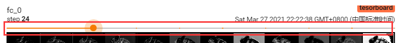
就以step=24为例说明，我们设置显示的列数等于通道数。而batch_size为4，且只显示前12个通道。因此下图共有4行12列，每一行分别代表每个batch的第一层卷积层的前12个通道图像。

在fc_0中还能看到大概的图像轮廓，下面看fc_3(依然查看step=24)。

fc_3依然能看出有图像的大概样子。再看fc_6的

fc_6好多特征图已经明显成黑色了，而且也看不到图像的轮廓了。所以深度越深数据越抽象。

如何在本地显示一个batch的图像?
在外部定义函数

import matplotlib.pyplot as plt
import numpy as np

def imshow(img):
   img = img / 2 + 0.5    #这是transform时的值全0.5时的反操作
   npimg = img.numpy()
   plt.imshow(np.transpose(npimg, (1, 2, 0))) 
   plt.show()

调用

image_batch = torchvision.utils.make_grid(images)
imshow(image_batch)

3. 网络模型的可视化

这个容易做，只需要在writer = SummaryWriter("runs/tesorboard")的下一行加上

writer.add_graph(net, torch.zeros([1,3,224,224]).to(device))

即可。然后打开GRAPHS标签，即可看到右边的网络模型图。

打开Main Graph下的每一项都有详细的说明，如AlexNet项。

上图显示了卷积fc层和全连接line层。再双击fc层可以看到它的更加详细的信息。

这和我们定义的网络一致。