How to Use the Torch Module in Pytorch to Quckily Build a Simple Two Layers Neural Network

1. Using numpy to show the detailed process of building the network

Here are some preparations to be done at the very beginning.

import numpy as np
N, D_in, H, D_out = 64, 1000, 100, 10
# N is the batch size; D_in is the input dimension;
# H is the hidden dimension; D_out is the output dimension.
x = np.random.randn(N, D_in)
y = np.random.randn(N, D_out)

As you see, we create random input and output data using the code above. Then we are supposed to initialize those weights in this neural network. Besides, in order to simplify the network, we let the bias be zero.

w1 = np.random.randn(D_in, H)
w2 = np.random.randn(H, D_out)

We set the learning rate at the same time.

learning_rate = 1e-6

Next, we are going to write the main part of the neural network.

for t in range(500):
    # Forward pass: compute the predicted values of y
    h = x.dot(w1)
    h_relu = np.maximum(h, 0)
    y_pred = h_relu.dot(w2)

500 is the iteration times of the loop. With the predicted value of y, we can compute the loss between y_pred and y.

    # Compute and print loss
    loss = np.square(y_pred - y).sum()
    print(t, loss)

Next comes the backpropagation process. In this part, we are going to compute the gradients of weights with respect to the loss above.

    # Backprop to compute gradients of w1 and w2 with respect to loss
    grad_y_pred = 2.0 * (y_pred - y)
    grad_w2 = h_relu.T.dot(grad_y_pred)
    grad_h_relu = grad_y_pred.dot(w2.T)
    grad_h = grad_h_relu.copy()
    grad_h[h < 0] = 0
    grad_w1 = x.T.dot(grad_h)

At the bottom of the loop body, we manually update the weights.

    # Update weights
    w1 -= learning_rate * grad_w1
    w2 -= learning_rate * grad_w2

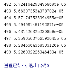
Here displays the result.


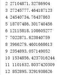
Apparently, the loss goes down to a very small value after 500 iterations.
We have to say that the training effect is quite thrilling.

2. Using torch to simplify the network

The code below is extracted from the complete process of building the neural network mentioned above with the help of the torch module. It is similar to the corresponding steps we proceed when we use the numpy module.

import torch

N, D_in, H, D_out = 64, 1000, 100, 10
x = torch.randn(N, D_in)
y = torch.randn(N, D_out)
w1 = torch.randn(D_in, H, requires_grad=True)
w2 = torch.randn(H, D_out, requires_grad=True)
# Only by making the statement "requires_grad=True"
# can you receive the gradients of weights.

learning_rate = 1e-6
for t in range(500):
    # Forward pass: compute predicted values of y
    y_pred = x.mm(w1).clamp(min=0).mm(w2)

    # Compute and print loss
    loss = (y_pred - y).pow(2).sum()
    print(t, loss.item())

The rest parts of building the neural network with torch are displayed below.

# Backward pass
    loss.backward()

    # Update weights using gradient descent
    with torch.no_grad():#In this way, the gradients won't take up space in memory
        w1 -= learning_rate * w1.grad
        w2 -= learning_rate * w2.grad
        #The tensors of gradients need to be set zero before
        #the next iteration, otherwise it keeps going up.
        w1.grad.zero_()
        w2.grad.zero_()

Surprisingly, “loss.backward()” represents the whole backpropagation process. Now the computer will automatically compute the gradients with respect to the loss above.
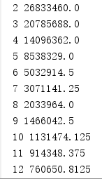
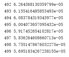
Here comes the result.

3. Using torch.nn to simplify the network

The preparation

import torch
import torch.nn as nn

N, D_in, H, D_out = 64, 1000, 100, 10
x = torch.randn(N, D_in)
y = torch.randn(N, D_out)

The code below is the most terrific part of the application of torch.nn.

model = torch.nn.Sequential(
    torch.nn.Linear(D_in, H, bias=False),
    torch.nn.ReLU(),
    torch.nn.Linear(H, D_out, bias=False),
)

Using “torch.nn.Sequential()”, we can build a model of the neural network in such a intuitive way.
Next, let me show you the rest of the code, and the final result running the code.

# improve the initialized condition
torch.nn.init.normal_(model[0].weight)
torch.nn.init.normal_(model[2].weight)

loss_fn = nn.MSELoss(reduction='sum')

learning_rate = 1e-6
for it in range(500):
    # Forward pass
    y_pred = model(x)

    # compute loss
    loss = loss_fn(y_pred, y)
    print(it, loss.item())

    # Backward pass
    loss.backward()

    # update weights of w1 and w2
    with torch.no_grad():
        for param in model.parameters():  # param (tensor, grad)
            param -= learning_rate * param.grad

    model.zero_grad()

With the comments displayed next to the code, I’m sure that you can understand what I’m doing.
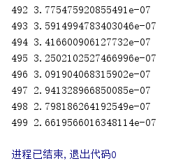
Here comes the result.

Apparently, the loss goes down to a very small value after 500 iterations.
The result excites me a lot.

4. Using optimizers to simplify the network

Using “loss.backward()” and “torch.nn.Sequential()” simplifies the process of building a neural network to a great extent. However, until now, we still have to update the weights manually. But don’t worry about that, after learning the usage of optimizers, you can solve the problem.

import torch
import torch.nn as nn

N, D_in, H, D_out = 64, 1000, 100, 10
x = torch.randn(N, D_in)
y = torch.randn(N, D_out)

model = torch.nn.Sequential(
    torch.nn.Linear(D_in, H, bias=False),
    torch.nn.ReLU(),
    torch.nn.Linear(H, D_out, bias=False),
)

import torch.nn as nn
import torch

N, D_in, H, D_out = 64, 1000, 100, 10

x = torch.randn(N, D_in)
y = torch.randn(N, D_out)

model = torch.nn.Sequential(
    torch.nn.Linear(D_in, H, bias=False),
    torch.nn.ReLU(),
    torch.nn.Linear(H, D_out, bias=False),
)

torch.nn.init.normal_(model[0].weight)
torch.nn.init.normal_(model[2].weight)

loss_fn = nn.MSELoss(reduction='sum')

There is almost no difference between the code above and the corresponding code in last part.
Next, we are going to learn the definition of an optimizer and how to update all parameters in one step.

learning_rate = 1e-6
optimizer = torch.optim.SGD(model.parameters(), lr=learning_rate)# the definition of an optimizer

Besides of SGD, you can use an optimizer called Adam as well. However, you need to change the learning_rate to 1e-4 at the same time in order to attain ideal training effect.

for it in range(500):
    # Forward pass
    y_pred = model(x)  # model.forward()

    # compute loss
    loss = loss_fn(y_pred, y)
    print(it, loss.item())

    optimizer.zero_grad()
    # Backward pass
    loss.backward()

    # update model parameters
    optimizer.step()# update all parameters in one step

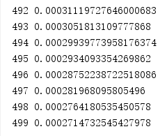
Here comes the result.

The training effect is satisfying.
All pains, all gains.