Use Data in Sklearn to Make a Diabetes Prediction

About Sklearn

Sklearn, also called Scikit-learn, is a third party module commonly used in machine learning, which encapsulates the commonly used machine learning methods, including Regression, Dimensionality Reduction, Classfication, Clustering, etc.
Sklearn provides some standard data, so we don’t have to look for data from other websites for training.

Data of This Experiment

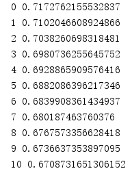
In this experiment, we use one of the standard data stored in sklearn which is named diabetes.csv.gz. And the picture below shows part of the data.
A row is a sample. And one sample contains nine features. I intend to label the first eight features as x1 through x8. And the feature in the last column will be labeled y, where 0 means not having diabetes and 1 means having diabetes. Apparently, this is a classification problem.

Code of This Experiment

Prepare dataset.

import numpy as np
import torch
xy = np.loadtxt('diabetes.csv.gz', delimiter=',', dtype=np.float32)
x_data = torch.from_numpy(xy[:,:-1])
y_data = torch.from_numpy(xy[:, [-1]])#input as a tensor

Design model using class which inherits from torch.nn.Module.

class Model(torch.nn.Module):
     def __init__(self):
         super(Model, self).__init__()
         self.linear1 = torch.nn.Linear(8, 6)
         #8 is the dimension of input.
         #6 is the dimension of output.
         self.linear2 = torch.nn.Linear(6, 4)
         self.linear3 = torch.nn.Linear(4, 1)
         self.sigmoid = torch.nn.Sigmoid()

     def forward(self, x):
         x = self.sigmoid(self.linear1(x))
         x = self.sigmoid(self.linear2(x))
         x = self.sigmoid(self.linear3(x))
         return x

model = Model()

Construct loss and optimizer. Since it’s a classification problem, I choose BCELoss() to calculate the loss.

criterion = torch.nn.BCELoss(size_average=True)
optimizer = torch.optim.SGD(model.parameters(), lr=0.1)

Here comes the training cycle.

for epoch in range(1000):
    # Forward
    y_pred = model(x_data)
    loss = criterion(y_pred, y_data)
    print(epoch, loss.item())
    # Backward
    optimizer.zero_grad()
    loss.backward()
    # Update
    optimizer.step()

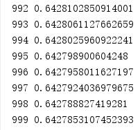
Here comes the result.

Improvement

Based on the code displayed in last part, I intend to try different activate functions and see the effect.
Here are graphs of several activate functions.

From these graphs, it’s not hard to see that only Sigmoid Function is limited to between 0 and 1. Besides, the curve of Softplus Function is similar to the one of ReLu Function.
First, I will replace Sigmoid with ReLu.
The following code only shows the different part. The rest of the code is totally the same as the former one.

class Model(torch.nn.Module):
     def __init__(self):
         super(Model, self).__init__()
         self.linear1 = torch.nn.Linear(8, 6)
         self.linear2 = torch.nn.Linear(6, 4)
         self.linear3 = torch.nn.Linear(4, 1)
         self.activate = torch.nn.ReLU()

     def forward(self, x):
         x = self.activate(self.linear1(x))
         x = self.activate(self.linear2(x))
         x = self.activate(self.linear3(x))
         return x

model = Model()

Here comes the result.

The reason is that the input of BCELoss() should be decimals from 0 to 1, however, the output of ReLu() may go beyond the range.
From the former content, we know that Sigmoid Function is limited to between 0 and 1. Therefore, we can use it as the activate function of the last layer to avoid the error above.
Here comes the code.

class Model(torch.nn.Module):
     def __init__(self):
         super(Model, self).__init__()
         self.linear1 = torch.nn.Linear(8, 6)
         self.linear2 = torch.nn.Linear(6, 4)
         self.linear3 = torch.nn.Linear(4, 1)
         self.activate = torch.nn.ReLU()
         self.sigmoid = torch.nn.Sigmoid()

     def forward(self, x):
         x = self.activate(self.linear1(x))
         x = self.activate(self.linear2(x))
         x = self.sigmoid(self.linear3(x))
         return x

Here come the result.

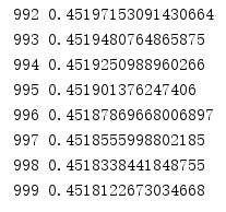
The loss becomes smaller compared to the former result. I do make an improvement.
Next, I will try Softplus.

import numpy as np
import torch
import torch.nn.functional as F
xy = np.loadtxt('diabetes.csv.gz', delimiter=',', dtype=np.float32)
x_data = torch.from_numpy(xy[:,:-1])
y_data = torch.from_numpy(xy[:, [-1]])

class Model(torch.nn.Module):
     def __init__(self):
         super(Model, self).__init__()
         self.linear1 = torch.nn.Linear(8, 6)
         self.linear2 = torch.nn.Linear(6, 4)
         self.linear3 = torch.nn.Linear(4, 1)
         self.activate = F.softplus
         self.sigmoid = torch.nn.Sigmoid()

     def forward(self, x):
         x = self.activate(self.linear1(x))
         x = self.activate(self.linear2(x))
         x = self.sigmoid(self.linear3(x))
         return x

Here comes the result.

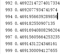
Compared to the result of only using Sigmoid, it does make an improvement. But in this experiment, it doesn’t show any superiority compared to ReLu.

That’s all. Thanks for your attention.