轻量级CNN网络之MobileNetv2

---

MobileNet网络是Google提出主要应用在移动端的轻量级CNN网络，之前的文章（CNN模型之MobileNet）已经对MobileNetv1版本进行了详细的介绍。目前，Google已经公开了MobileNetv2，它相比v1更高效。MobileNetv2依然使用v1中的depthwise separable convolution，区别在于v2又引入了残差结构和bottleneck层，这种新的结构称为Bottleneck residual block。

Depthwise Separable Convolution

Depthwise Separable Convolution是MobileNetv1所采用的核心结构，如图 1所示，它包含一个depthwise卷积和1x1卷积（或者称为pointwise卷积），这种结构将空间相关性和通道相关性分离（见Xception文章），相比传统的卷积，它可以减少约$k^2$计算复杂度，当卷积核$k=3$时，大约比原来计算花费少8~9倍，但是却在准确度方面损失很少。MobileNetv2作为v1的升级版，也主要采用Depthwise Separable Convolution结构。

图1 Depthwise Separable Convolution结构

Linear Bottlenecks

对于CNN网络某一层$L_i$的特征图，其维度大小为$h_i\times w_i\times d_i$，我们感兴趣的是它的核心信息，这里称为“主要流形”（manifold of interest）。而“主要流形”是可以用一个低维度空间来表达的。这实际上是说神经网络某层特征，其主要信息可以用一个低维度特征来表征。据此，我们可以在网络引入“bottlenck layer”来表征某一个深层特征的“主要流形”，作者发现这个“bottlenck layer”最好采用线性激活，而不是采用ReLU，因为在“bottlenck layer”采用非线性激活会损失很多信息，毕竟特征已经在低维度空间（paper中有理论分析和实验证明）。在Depthwise Separable Convolution引入“bottlenck layer”后，结构如图2所示，其中浅色代表的是下一个block的开始，并且注意方块代表的是特征图，而红色映射才是卷积或者ReLU操作。图2-a是常规的卷积，而图2-b是Depthwise Separable Convolution，这在MobileNetv1中大量使用。当在Depthwise Separable Convolution后面加入“bottlenck layer”就变成了图2-c，但是考虑到block是互相堆积的，调整一下视角，如果将“bottlenck layer”看成block的输入，那么这种结构也等价于图2-d。对于图2-d，block中开始的1x1卷积层称为“expansion layer”，它的通道大小（inner size）和输入bottleneck层的通道大小之比，称为扩展比（expansion ratio）。扩展层之后是depthwise卷积，然后采用1x1卷积得到block的输出特征，这个卷积后面没有非线性激活。对于图2-d这种结构，block的输入和输出特征是bottleneck特征，所以这个block称为bottleneck block，至于为什么要采用图2-d的视角，而不是图2-c，后面会有说明。

图2 加入linear bottlenecks的Depthwise Separable Convolution

Inverted Residuals

当我们在上面的block中加入短路连接，它就变成了残差结构，但是这个shortcut connection是在bottlenecks之间。这与常规的残差block是相反的，因为residual block一般先采用bottleneck layer进行降维，最后进行扩展。两者的差异如图3所示，可以看到两者的bottleneck的位置恰恰相反，paper里面称这种相反的残差block为inverted residual block。前面也说了，大家可能会疑惑为什么要采用这种相反的结构呢，paper说这种结果可以在实现上减少内存的使用，这点paper里面有详细的说明，另外一点是这种相反的结构从实验结果上也更好一点。

图3 inverted residual block和residual block之间的对比

网络结构

前面我们讲了MobileNetv2相比v1的两个主要改进：linear bottleneck和inverted residual。改进后的新结构称为bottleneck residual block，表1给出了这个block的内部结构，其中t是扩展比。

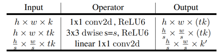
表1 Bottleneck residual block的内部构成

Bottleneck residual block其实包含3层卷积操作，图4更直观的给出了block的内部结构。首先是一个1x1的卷积，称为expansion layer，它将输入的通道维度从k变换为tk，在实际中t取大于1的值最有效，paper里面的默认值t=6。然后是3x3的depthwise conv，每个通道上是单独卷积的。最后是一个projection layer，它将得到block的输入特征，一般情形下是降低通道大小的，所以是bottleneck layer，如前面所述，bottleneck后面没有采用非线性激活。这种结构一个有意思的特征是它将网络的容量（capacity）和表达力（expressiveness）分离开来。其中bottleneck layer负责的是输入和输出之间的转换，这可以看成capacity，而中间的expansion layer充当的是非线性变换，可以看成是expressiveness。

图4 Bottleneck residual block示意图

这篇博客（MobileNet version 2）对这种结构给出了一个有趣的解释，如5所示。其中expansion layer可以看做解压器，类似unzip，将特征恢复到高维空间，而
depthwise layer可以看成过滤器，筛选比较重要的特征，最后projection layer将其压缩到低维空间。

图5 Bottleneck residual block的另一种解释

MobileNetv2与其它网络的对比如图6所示，值得注意的对于stride=2的block没有采用残差结构。

图6 MobileNetv2与其它网络的结构对比

将block堆积起来，就形成最终的MobileNetv2网络，各个block设计如表2所示，其中t是扩展比，c是block的输出特征的channel大小，n是block的重复次数，s是stride，注意只有对于重复的block只有开始的s才是2。另外与MobileNetv1类似，v2也设计了width multiplier和输入大小两个超参数控制网络的参数量，表2中默认的是width multiplier=1.0，输入大小是224x224。输入大小影响的是特征图空间大小，而width multiplier影响的是特征图channel大小。输入大小可以从96到224，而width multiplier可以从0.35到1.4。值得注意的一点是当width multiplier小于1时，不对最后一个卷积层的channel进行调整以保证性能，即维持1280。

表2 MobileNetv2的网络结构

MobileNetv2在ImageNet上分类效果与其它网络对比如表3所示，可以看到在同样参数大小下，MobileNetv2比MobileNetv1和ShuffleNet要好，而且速度也更快一些。另外MobileNetv2还可以应用在语义分割（DeepLab）和目标检测（SSD）中，也得到了较好的结果。

表3 MobileNetv2与其它网络在ImageNet上的对比

TensorFlow上的实现

Google已经开源了MobileNetv2的代码，其基于TensorFlow/slim框架实现，slim是一个较好的CNN轻量级框架。这里给出简化版本的实现。

对于MobileNetv2的实际实现中，会对channel进行一些限制，如保证channel的最小值以及是8的倍数，所以会存在如下的辅助函数：

    def _make_divisible(v, divisor, min_value=None):
        """make `v` is divided exactly by `divisor`, but keep the min_value"""
        if min_value is None:
            min_value = divisor
        new_v = max(min_value, int(v + divisor / 2) // divisor * divisor)
        # Make sure that round down does not go down by more than 10%.
        if new_v < 0.9 * v:
            new_v += divisor
        return new_v
    
    
    @slim.add_arg_scope
    def _depth_multiplier_func(params,
                               multiplier,
                               divisible_by=8,
                               min_depth=8):
        """get the new channles"""
        if 'num_outputs' not in params:
            return
        d = params['num_outputs']
        params['num_outputs'] = _make_divisible(d * multiplier, divisible_by,
                                                       min_depth)
              

这些对于通过width multiplier改变channel大小做了一定的限制。然后我们实现网络最核心的结构Bottleneck residual block：

    @slim.add_arg_scope
    def expanded_conv(x,
                      num_outputs,
                      expansion=6,
                      stride=1,
                      rate=1,
                      normalizer_fn=slim.batch_norm,
                      project_activation_fn=tf.identity,
                      padding="SAME",
                      scope=None):
        """The expand conv op in MobileNetv2
            1x1 conv -> depthwise 3x3 conv -> 1x1 linear conv
        """
        with tf.variable_scope(scope, default_name="expanded_conv") as s, \
           tf.name_scope(s.original_name_scope):
            prev_depth = x.get_shape().as_list()[3]
            # the filters of expanded conv
            inner_size = prev_depth * expansion
            net = x
            # only inner_size > prev_depth, use expanded conv
            if inner_size > prev_depth:
                net = slim.conv2d(net, inner_size, 1, normalizer_fn=normalizer_fn,
                                  scope="expand")
            # depthwise conv
            net = slim.separable_conv2d(net, num_outputs=None, kernel_size=3,
                                        depth_multiplier=1, stride=stride,
                                        rate=rate, normalizer_fn=normalizer_fn,
                                        padding=padding, scope="depthwise")
            # projection
            net = slim.conv2d(net, num_outputs, 1, normalizer_fn=normalizer_fn,
                              activation_fn=project_activation_fn, scope="project")
    
            # residual connection
            if stride == 1 and net.get_shape().as_list()[-1] == prev_depth:
                net += x
    
            return net

这里的实现相比官方实现做了一定的简化，官方代码中包含很多灵活的参数，但是在实际中却没有采用，所以我选择了paper中的默认配置。注意这里的rate参数主要是为了配合语义分割模型，因为在DeepLab模型会采用空洞卷积来平衡特征图空间大小。

在定义网络之前，我们使用一个简单的Op类，对网络结构进行配置：

    _Op = namedtuple("Op", ['op', 'params', 'multiplier_func'])
    
    def op(op_func, **params):
        return _Op(op=op_func, params=params,
                   multiplier_func=_depth_multiplier_func)
    
    
    CONV_DEF = [op(slim.conv2d, num_outputs=32, stride=2, kernel_size=3),
                op(expanded_conv, num_outputs=16, expansion=1),
                op(expanded_conv, num_outputs=24, stride=2),
                op(expanded_conv, num_outputs=24, stride=1),
                op(expanded_conv, num_outputs=32, stride=2),
                op(expanded_conv, num_outputs=32, stride=1),
                op(expanded_conv, num_outputs=32, stride=1),
                op(expanded_conv, num_outputs=64, stride=2),
                op(expanded_conv, num_outputs=64, stride=1),
                op(expanded_conv, num_outputs=64, stride=1),
                op(expanded_conv, num_outputs=64, stride=1),
                op(expanded_conv, num_outputs=96, stride=1),
                op(expanded_conv, num_outputs=96, stride=1),
                op(expanded_conv, num_outputs=96, stride=1),
                op(expanded_conv, num_outputs=160, stride=2),
                op(expanded_conv, num_outputs=160, stride=1),
                op(expanded_conv, num_outputs=160, stride=1),
                op(expanded_conv, num_outputs=320, stride=1),
                op(slim.conv2d, num_outputs=1280, stride=1, kernel_size=1),
                ]

然后定义整个网络：

    def mobilenetv2(x,
                    num_classes=1001,
                    depth_multiplier=1.0,
                    scope='MobilenetV2',
                    finegrain_classification_mode=False,
                    min_depth=8,
                    divisible_by=8,
                    output_stride=None,
                    ):
        """Mobilenet v2
        Args:
            x: The input tensor
            num_classes: number of classes
            depth_multiplier: The multiplier applied to scale number of
                channels in each layer. Note: this is called depth multiplier in the
                paper but the name is kept for consistency with slim's model builder.
            scope: Scope of the operator
            finegrain_classification_mode: When set to True, the model
                will keep the last layer large even for small multipliers.
                The paper suggests that it improves performance for ImageNet-type of problems.
            min_depth: If provided, will ensure that all layers will have that
              many channels after application of depth multiplier.
           divisible_by: If provided will ensure that all layers # channels
              will be divisible by this number.
        """
        conv_defs = CONV_DEF
    
        # keep the last conv layer very larger channel
        if finegrain_classification_mode:
            conv_defs = copy.deepcopy(conv_defs)
            if depth_multiplier < 1:
                conv_defs[-1].params['num_outputs'] /= depth_multiplier
    
        depth_args = {}
        # NB: do not set depth_args unless they are provided to avoid overriding
        # whatever default depth_multiplier might have thanks to arg_scope.
        if min_depth is not None:
            depth_args['min_depth'] = min_depth
        if divisible_by is not None:
            depth_args['divisible_by'] = divisible_by
    
        with slim.arg_scope([_depth_multiplier_func], **depth_args):
            with tf.variable_scope(scope, default_name='Mobilenet'):
                # The current_stride variable keeps track of the output stride of the
                # activations, i.e., the running product of convolution strides up to the
                # current network layer. This allows us to invoke atrous convolution
                # whenever applying the next convolution would result in the activations
                # having output stride larger than the target output_stride.
                current_stride = 1
    
                # The atrous convolution rate parameter.
                rate = 1
    
                net = x
                # Insert default parameters before the base scope which includes
                # any custom overrides set in mobilenet.
                end_points = {}
                scopes = {}
                for i, opdef in enumerate(conv_defs):
                    params = dict(opdef.params)
                    opdef.multiplier_func(params, depth_multiplier)
                    stride = params.get('stride', 1)
                    if output_stride is not None and current_stride == output_stride:
                        # If we have reached the target output_stride, then we need to employ
                        # atrous convolution with stride=1 and multiply the atrous rate by the
                        # current unit's stride for use in subsequent layers.
                        layer_stride = 1
                        layer_rate = rate
                        rate *= stride
                    else:
                        layer_stride = stride
                        layer_rate = 1
                        current_stride *= stride
                    # Update params.
                    params['stride'] = layer_stride
                    # Only insert rate to params if rate > 1.
                    if layer_rate > 1:
                        params['rate'] = layer_rate
    
                    try:
                        net = opdef.op(net, **params)
                    except Exception:
                        raise ValueError('Failed to create op %i: %r params: %r' % (i, opdef, params))
    
                with tf.variable_scope('Logits'):
                    net = global_pool(net)
                    end_points['global_pool'] = net
                    if not num_classes:
                        return net, end_points
                    net = slim.dropout(net, scope='Dropout')
                    # 1 x 1 x num_classes
                    # Note: legacy scope name.
                    logits = slim.conv2d(
                        net,
                        num_classes, [1, 1],
                        activation_fn=None,
                        normalizer_fn=None,
                        biases_initializer=tf.zeros_initializer(),
                        scope='Conv2d_1c_1x1')
    
                    logits = tf.squeeze(logits, [1, 2])
    
                    return logits

注意output_stride参数是配合语义分割模型，在DeepLab中output_stride取8或者16，它表示的是特征图最高下采样率，当超过这个值时，采用空洞卷积。

其它的模型超参数，我们可以通过slim的arg_scope来控制，这是slim框架我最喜欢的一个功能：

    def mobilenet_arg_scope(is_training=True,
                            weight_decay=0.00004,
                            stddev=0.09,
                            dropout_keep_prob=0.8,
                            bn_decay=0.997):
        """Defines Mobilenet default arg scope.
        Usage:
         with tf.contrib.slim.arg_scope(mobilenet.training_scope()):
           logits, endpoints = mobilenet_v2.mobilenet(input_tensor)
         # the network created will be trainble with dropout/batch norm
         # initialized appropriately.
        Args:
            is_training: if set to False this will ensure that all customizations are
                set to non-training mode. This might be helpful for code that is reused
            across both training/evaluation, but most of the time training_scope with
            value False is not needed. If this is set to None, the parameters is not
            added to the batch_norm arg_scope.
            weight_decay: The weight decay to use for regularizing the model.
            stddev: Standard deviation for initialization, if negative uses xavier.
            dropout_keep_prob: dropout keep probability (not set if equals to None).
            bn_decay: decay for the batch norm moving averages (not set if equals to
                None).
        Returns:
            An argument scope to use via arg_scope.
        """
        # Note: do not introduce parameters that would change the inference
        # model here (for example whether to use bias), modify conv_def instead.
        batch_norm_params = {
            'center': True,
            'scale': True,
            'decay': bn_decay,
            'is_training': is_training
        }
        if stddev < 0:
            weight_intitializer = slim.initializers.xavier_initializer()
        else:
            weight_intitializer = tf.truncated_normal_initializer(stddev=stddev)
    
        # Set weight_decay for weights in Conv and FC layers.
        with slim.arg_scope(
            [slim.conv2d, slim.fully_connected, slim.separable_conv2d],
            weights_initializer=weight_intitializer,
            normalizer_fn=slim.batch_norm,
            activation_fn=tf.nn.relu6), \
            slim.arg_scope([slim.batch_norm], **batch_norm_params), \
            slim.arg_scope([slim.dropout], is_training=is_training,
                         keep_prob=dropout_keep_prob), \
            slim.arg_scope([slim.conv2d, slim.separable_conv2d],
                           biases_initializer=None,
                           padding="SAME"), \
            slim.arg_scope([slim.conv2d],
                         weights_regularizer=slim.l2_regularizer(weight_decay)), \
            slim.arg_scope([slim.separable_conv2d], weights_regularizer=None) as s:
            return s

最后可以通过如下代码测试模型（预训练模型官方实现中已经给出）：

        inputs = tf.placeholder(tf.uint8, [None, None, 3])
        images = tf.expand_dims(inputs, 0)
        images = tf.cast(images, tf.float32) / 128. - 1
        images.set_shape((None, None, None, 3))
        images = tf.image.resize_images(images, (224, 224))
    
        with slim.arg_scope(mobilenet_arg_scope(is_training=False)):
            logits = mobilenetv2(images)
    
        # Restore using exponential moving average since it produces (1.5-2%) higher
        # accuracy
        ema = tf.train.ExponentialMovingAverage(0.999)
        vars = ema.variables_to_restore()
    
        saver = tf.train.Saver(vars)
    
        print(len(tf.global_variables()))
        for var in tf.global_variables():
            print(var)
        checkpoint_path = ""
        image_file = ""
        with tf.Session() as sess:
            saver.restore(sess, checkpoint_path)
    
            img = cv2.imread(image_file)
            img = cv2.cvtColor(img, cv2.COLOR_BGR2RGB)
    
            print(np.argmax(sess.run(logits, feed_dict={inputs: img})[0]))

整个实现代码可以见我的GitHub（xiaohu2015/DeepLearning_tutorials），欢迎star。

小结

这里比较简单地介绍了MobileNetv2，相比v1其核心区别就在于bottleneck和residual结构。但是，对于paper里面一些理论分析这里没有给出，感兴趣的可以自己啃一下。

参考

1. MobileNetV2: Inverted Residuals and Linear Bottlenecks
2. MobileNet version 2 （部分图来源这个blog）
3. MobileNetv2的官方代码