回归----非线性逻辑回归

目录

梯度下降法实现非线性逻辑回归代码

sklearn实现非线性逻辑回归代码

---

非线性逻辑回归和线性逻辑回归原理差不多，但是非线性逻辑回归的决策边界是一条曲线

梯度下降法实现非线性逻辑回归代码

• 导入所用的包

import numpy as np
import matplotlib.pyplot as plt
from sklearn.metrics import classification_report  #对模型进行评估
from sklearn import preprocessing  #对数据做标准化
from sklearn.preprocessing import  PolynomialFeatures
#数据是否需要标准化
scale = False
%matplotlib inline

•  导入数据对数据进行处理，画散点图

data = np.genfromtxt('LR-testSet2.txt',delimiter = ',')
x_data = data[:,:-1]
y_data = data[:,-1,np.newaxis]

def plot():
    x0 = []
    y0 = []
    x1 = []
    y1 = []
    
    for i in range(len(x_data)):
        if y_data[i] == 0:
            x0.append(x_data[i,0])
            y0.append(x_data[i,1])
        else:
            x1.append(x_data[i,0])
            y1.append(x_data[i,1])
    
    #画图
    scatter0 = plt.scatter(x0,y0,c='y',marker='o')
    scatter1 = plt.scatter(x1,y1,c='g',marker='x')
    #画图例
    plt.legend(handles = [scatter0,scatter1],labels=['label0','label1'],loc ='best')
    
plot()
plt.show()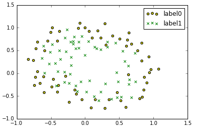

  

• 定义多项式回归 

#定义多项式回归，degree的值可以调节多项式的特征
poly_reg = PolynomialFeatures(degree = 3) 
#特征处理
x_poly = poly_reg.fit_transform(x_data)  #degree = 3   x_poly  =  x^0  x^1  x^2  x^3

• 实现sigmoid函数以及代价函数

def sigmoid(x):
    return 1.0/(1+np.exp(-x))

def cost(Xmat,Ymat,ws):
    left  = np.multiply(Ymat,np.log(sigmoid(Xmat*ws)))
    right = np.multiply(1-Ymat,np.log(1-sigmoid(Xmat*ws)))
    return np.sum(left+right) / -(len(Xmat))

def gradAscent(Xarr,Yarr):
    
    if scale == True:
        Xarr = preprocessing.scale(Xarr)
    Xmat = np.mat(Xarr)
    Ymat = np.mat(Yarr)
    
    lr = 0.03
    epochs  =50000
    costList = []
    
    m,n = np.shape(Xmat) #行代表数据的个数，列代表权值的个数
    ws = np.mat(np.ones((n,1))) #初始化权值
    
    for i in range(epochs+1):
        h = sigmoid(Xmat*ws)
        ws_grad = Xmat.T*(h - Ymat)/m
        ws = ws - lr *ws_grad
        
        if i % 50 ==0:
            costList.append(cost(Xmat,Ymat,ws))
        
    return ws,costList

• 调用函数

ws,costList = gradAscent(x_poly,y_data)

• 画图 

x_min,x_max = x_data[:,0].min() -1,x_data[:,0].max()+1
y_min,y_max = x_data[:,1].min() -1,x_data[:,1].max()+1

#生成网格矩阵
xx,yy = np.meshgrid(np.arange(x_min,x_max,0.02),np.arange(y_min,y_max,0.02))

z = sigmoid(poly_reg.fit_transform(np.c_[xx.ravel(),yy.ravel()]).dot(np.array(ws)))
for i in range(len(z)):
    if z[i] > 0.5:
        z[i] = 1
    else:
        z[i] = 0
        
z = z.reshape(xx.shape)
#画等高线图
cs = plt.contourf(xx,yy,z)
plot()
plt.show()
    

  

• 做预测 

def predict(x_data,ws):
#     if scale == True:
#       x_data = preprocessing.scale(x_data)
     Xmat = np.mat(x_data)
     ws = np.mat(ws)
     return [1 if x >= 0.5 else 0 for x in sigmoid(Xmat*ws)]

predictions = predict(x_poly,ws)

print(classification_report(y_data,predictions))

预测结果： 

sklearn实现非线性逻辑回归代码

• 导入所用的包 

import numpy as np
import matplotlib.pyplot as plt
from sklearn import linear_model
from sklearn.metrics import classification_report 
from sklearn.datasets import make_gaussian_quantiles
from sklearn.preprocessing import PolynomialFeatures
%matplotlib inline

• 随机生成散点，打印出 

x_data,y_data = make_gaussian_quantiles(n_samples = 500,n_features = 2,n_classes =2)
plt.scatter(x_data[:,0],x_data[:,1],c=y_data)
plt.show()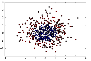

 

•  训练模型

logistic = linear_model.LogisticRegression()
logistic.fit(x_data,y_data)

• 画图 ，做预测

x_min,x_max = x_data[:,0].min() -1,x_data[:,0].max()+1
y_min,y_max = x_data[:,1].min() -1,x_data[:,1].max()+1

#生成网格矩阵
xx,yy = np.meshgrid(np.arange(x_min,x_max,0.02),np.arange(y_min,y_max,0.02))

z = logistic.predict(np.c_[xx.ravel(),yy.ravel()])       
z = z.reshape(xx.shape)
#画等高线图
cs = plt.contourf(xx,yy,z)
plt.scatter(x_data[:,0],x_data[:,1],c=y_data)
plt.show()

print('score:',logistic.score(x_data,y_data))

predictions = logistic.predict(x_poly)

print(classification_report(y_data,predictions))

 

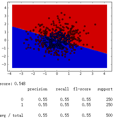
我们可以看到，在没有定义多项式回归，决策边界是一条直线，准确率只有0.55 

• 定义多项式回归 ，画图，做预测

#定义多项式回归，degree的值可以调节多项式的特征
poly_reg = PolynomialFeatures(degree = 5) 
#特征处理
x_poly = poly_reg.fit_transform(x_data)  #degree = 3   x_poly  =  x^0  x^1  x^2  x^3
logistic = linear_model.LogisticRegression()
logistic.fit(x_poly,y_data)

x_min,x_max = x_data[:,0].min() -1,x_data[:,0].max()+1
y_min,y_max = x_data[:,1].min() -1,x_data[:,1].max()+1

#生成网格矩阵
xx,yy = np.meshgrid(np.arange(x_min,x_max,0.02),np.arange(y_min,y_max,0.02))

z = logistic.predict(poly_reg.fit_transform(np.c_[xx.ravel(), yy.ravel()]))     
z = z.reshape(xx.shape)
#画等高线图
cs = plt.contourf(xx,yy,z)
plt.scatter(x_data[:,0],x_data[:,1],c=y_data)
plt.show()
print('score:',logistic.score(x_poly,y_data))
predictions = logistic.predict(x_poly)

print(classification_report(y_data,predictions))

如上图，我们可以看到，决策边界是一条曲线，准确率达到了0.98。