Andrew Ng Deep Learning 第二周 编程练习 Logistic regression with neural networks

Exercise 1

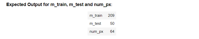
Find the values for:

• m_train (number of training examples)
• m_test (number of test examples)
• num_px (= height = width of a training image)
• Remember that train_set_x_orig is a numpy-array of shape (m_train, num_px, num_px, 3).
• For instance, you can access m_train by writing train_set_x_orig.shape[0]
  shape[0]:样本数量
  shape[1]:length
  shape[2]:height
  shape[3]:通道数
  

#(≈ 3 lines of code)
# m_train = 
# m_test = 
# num_px = 
# YOUR CODE STARTS HERE
m_train = train_set_x_orig.shape[0]
m_test = test_set_x_orig.shape[0]
num_px = train_set_x_orig.shape[2]
# YOUR CODE ENDS HERE

print ("Number of training examples: m_train = " + str(m_train))
print ("Number of testing examples: m_test = " + str(m_test))
print ("Height/Width of each image: num_px = " + str(num_px))
print ("Each image is of size: (" + str(num_px) + ", " + str(num_px) + ", 3)")
print ("train_set_x shape: " + str(train_set_x_orig.shape))
print ("train_set_y shape: " + str(train_set_y.shape))
print ("test_set_x shape: " + str(test_set_x_orig.shape))
print ("test_set_y shape: " + str(test_set_y.shape))

Exercise 2

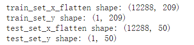
Reshape the training and test data sets so that images of size (num_px, num_px, 3) are flattened into single vectors of shape (num_px ∗ num_px ∗ 3, 1).

A trick when you want to flatten a matrix X of shape (a,b,c,d) to a matrix X_flatten of shape (b ∗ c ∗ d, a) is to use:

X_flatten = X.reshape(X.shape[0], -1).T # X.T is the transpose of X
利用他这里提供的快捷方式写

# Reshape the training and test examples
#(≈ 2 lines of code)
# train_set_x_flatten = ...
# test_set_x_flatten = ...
# YOUR CODE STARTS HERE
train_set_x_flatten = train_set_x_orig.reshape(train_set_x_orig.shape[0], -1).T 
test_set_x_flatten = test_set_x_orig.reshape(test_set_x_orig.shape[0], -1).T
 
# YOUR CODE ENDS HERE

# Check that the first 10 pixels of the second image are in the correct place
assert np.alltrue(train_set_x_flatten[0:10, 1] == [196, 192, 190, 193, 186, 182, 188, 179, 174, 213]), "Wrong solution. Use (X.shape[0], -1).T."
assert np.alltrue(test_set_x_flatten[0:10, 1] == [115, 110, 111, 137, 129, 129, 155, 146, 145, 159]), "Wrong solution. Use (X.shape[0], -1).T."

print ("train_set_x_flatten shape: " + str(train_set_x_flatten.shape))
print ("train_set_y shape: " + str(train_set_y.shape))
print ("test_set_x_flatten shape: " + str(test_set_x_flatten.shape))
print ("test_set_y shape: " + str(test_set_y.shape))

Exercise 3 sigmoid

第一周编程练习中已写过

# GRADED FUNCTION: sigmoid

def sigmoid(z):
    """
    Compute the sigmoid of z

    Arguments:
    z -- A scalar or numpy array of any size.

    Return:
    s -- sigmoid(z)
    """

    #(≈ 1 line of code)
    # s = ...
    # YOUR CODE STARTS HERE
    s = 1/(1 + np.exp(-z)) 
    
    # YOUR CODE ENDS HERE
    
    return s

Exercise 4 initialize_with_zeros

Implement parameter initialization in the cell below. You have to initialize w as a vector of zeros. If you don’t know what numpy function to use, look up np.zeros() in the Numpy library’s documentation.
w利用np.zeros进行初始化
b直接写成0.0就可以，因为python的boardcasting机制，但是注意，必须是浮点数，所以写成0.0

# GRADED FUNCTION: initialize_with_zeros

def initialize_with_zeros(dim):
    """
    This function creates a vector of zeros of shape (dim, 1) for w and initializes b to 0.
    
    Argument:
    dim -- size of the w vector we want (or number of parameters in this case)
    
    Returns:
    w -- initialized vector of shape (dim, 1)
    b -- initialized scalar (corresponds to the bias) of type float
    """
    
    # (≈ 2 lines of code)
    # w = ...
    # b = ...
    # YOUR CODE STARTS HERE
    w = np.zeros((dim,1))
    b = 0.0
    
    # YOUR CODE ENDS HERE

    return w, b

Exercise 5 propagate

Implement a function propagate() that computes the cost function and its gradient.
内容很简单，只要依照推导出的公式编程即可
但需要注意的是：
什么时候用的是矩阵乘法（np.dot）
什么时候用的是四则运算的乘法（*）

# GRADED FUNCTION: propagate

def propagate(w, b, X, Y):
    """
    Implement the cost function and its gradient for the propagation explained above

    Arguments:
    w -- weights, a numpy array of size (num_px * num_px * 3, 1)
    b -- bias, a scalar
    X -- data of size (num_px * num_px * 3, number of examples)
    Y -- true "label" vector (containing 0 if non-cat, 1 if cat) of size (1, number of examples)

    Return:
    cost -- negative log-likelihood cost for logistic regression
    dw -- gradient of the loss with respect to w, thus same shape as w
    db -- gradient of the loss with respect to b, thus same shape as b
    
    Tips:
    - Write your code step by step for the propagation. np.log(), np.dot()
    """
    
    m = X.shape[1]
    
    # FORWARD PROPAGATION (FROM X TO COST)
    #(≈ 2 lines of code)
    # compute activation
    # A = ...
    # compute cost by using np.dot to perform multiplication. 
    # And don't use loops for the sum.
    # cost = ...                                
    # YOUR CODE STARTS HERE
    A = sigmoid(np.dot(w.T,X)+b)
    cost = -np.sum(Y * np.log(A) + (1-Y) * np.log(1-A))/m
    
    # YOUR CODE ENDS HERE

    # BACKWARD PROPAGATION (TO FIND GRAD)
    #(≈ 2 lines of code)
    # dw = ...
    # db = ...
    # YOUR CODE STARTS HERE
    dw = np.dot(X,(A-Y).T) / m
    db = np.sum(A-Y) / m
    
    # YOUR CODE ENDS HERE
    cost = np.squeeze(np.array(cost))

    
    grads = {"dw": dw,
             "db": db}
    
    return grads, cost

Exercise 6 optimize

Write down the optimization function. The goal is to learn 𝑤 and 𝑏 by minimizing the cost function 𝐽 . For a parameter 𝜃 , the update rule is 𝜃=𝜃−𝛼 𝑑𝜃 , where 𝛼 is the learning rate.
利用梯度下降算法，计算最佳的w和b

# GRADED FUNCTION: optimize

def optimize(w, b, X, Y, num_iterations=100, learning_rate=0.009, print_cost=False):
    """
    This function optimizes w and b by running a gradient descent algorithm
    
    Arguments:
    w -- weights, a numpy array of size (num_px * num_px * 3, 1)
    b -- bias, a scalar
    X -- data of shape (num_px * num_px * 3, number of examples)
    Y -- true "label" vector (containing 0 if non-cat, 1 if cat), of shape (1, number of examples)
    num_iterations -- number of iterations of the optimization loop
    learning_rate -- learning rate of the gradient descent update rule
    print_cost -- True to print the loss every 100 steps
    
    Returns:
    params -- dictionary containing the weights w and bias b
    grads -- dictionary containing the gradients of the weights and bias with respect to the cost function
    costs -- list of all the costs computed during the optimization, this will be used to plot the learning curve.
    
    Tips:
    You basically need to write down two steps and iterate through them:
        1) Calculate the cost and the gradient for the current parameters. Use propagate().
        2) Update the parameters using gradient descent rule for w and b.
    """
    
    w = copy.deepcopy(w)
    b = copy.deepcopy(b)
    
    costs = []
    
    for i in range(num_iterations):
        # (≈ 1 lines of code)
        # Cost and gradient calculation 
        # grads, cost = ...
        # YOUR CODE STARTS HERE
        grads, cost = propagate(w, b, X, Y)
        
        # YOUR CODE ENDS HERE
        
        # Retrieve derivatives from grads
        dw = grads["dw"]
        db = grads["db"]
        
        # update rule (≈ 2 lines of code)
        # w = ...
        # b = ...
        # YOUR CODE STARTS HERE
        w = w - learning_rate * dw
        b = b - learning_rate * db
        
        
        # YOUR CODE ENDS HERE
        
        # Record the costs
        if i % 100 == 0:
            costs.append(cost)
        
            # Print the cost every 100 training iterations
            if print_cost:
                print ("Cost after iteration %i: %f" %(i, cost))
    
    params = {"w": w,
              "b": b}
    
    grads = {"dw": dw,
             "db": db}
    
    return params, grads, costs

Exercise 7 predict

The previous function will output the learned w and b. We are able to use w and b to predict the labels for a dataset X. Implement the predict() function. There are two steps to computing predictions:

# GRADED FUNCTION: predict

def predict(w, b, X):
    '''
    Predict whether the label is 0 or 1 using learned logistic regression parameters (w, b)
    
    Arguments:
    w -- weights, a numpy array of size (num_px * num_px * 3, 1)
    b -- bias, a scalar
    X -- data of size (num_px * num_px * 3, number of examples)
    
    Returns:
    Y_prediction -- a numpy array (vector) containing all predictions (0/1) for the examples in X
    '''
    
    m = X.shape[1]
    Y_prediction = np.zeros((1, m))
    w = w.reshape(X.shape[0], 1)
    
    # Compute vector "A" predicting the probabilities of a cat being present in the picture
    #(≈ 1 line of code)
    # A = ...
    # YOUR CODE STARTS HERE
    A = np.dot(w.T,X) + b
    
    # YOUR CODE ENDS HERE
    
    for i in range(A.shape[1]):
        
        # Convert probabilities A[0,i] to actual predictions p[0,i]
        #(≈ 4 lines of code)
        # if A[0, i] > ____ :
        #     Y_prediction[0,i] = 
        # else:
        #     Y_prediction[0,i] = 
        # YOUR CODE STARTS HERE
        if A[0, i] >  0:
             Y_prediction[0,i] = 1
        else:
             Y_prediction[0,i] = 0
        
        
        # YOUR CODE ENDS HERE
    
    return Y_prediction

Exercise 8 model

Implement the model function.
Use the following notation:

• Y_prediction_test for your predictions on the test set
• Y_prediction_train for your predictions on the train set
• parameters, grads, costs for the outputs of optimize()

# GRADED FUNCTION: model

def model(X_train, Y_train, X_test, Y_test, num_iterations=2000, learning_rate=0.5, print_cost=False):
    """
    Builds the logistic regression model by calling the function you've implemented previously
    
    Arguments:
    X_train -- training set represented by a numpy array of shape (num_px * num_px * 3, m_train)
    Y_train -- training labels represented by a numpy array (vector) of shape (1, m_train)
    X_test -- test set represented by a numpy array of shape (num_px * num_px * 3, m_test)
    Y_test -- test labels represented by a numpy array (vector) of shape (1, m_test)
    num_iterations -- hyperparameter representing the number of iterations to optimize the parameters
    learning_rate -- hyperparameter representing the learning rate used in the update rule of optimize()
    print_cost -- Set to True to print the cost every 100 iterations
    
    Returns:
    d -- dictionary containing information about the model.
    """
    # (≈ 1 line of code)   
    # initialize parameters with zeros 
    # w, b = ...
    w,b  = np.zeros((X_train.shape[0],1)), 0.0
    
    #(≈ 1 line of code)
    # Gradient descent 
    # params, grads, costs = ...
    
    # Retrieve parameters w and b from dictionary "params"
    # w = ...
    # b = ...
    
    # Predict test/train set examples (≈ 2 lines of code)
    # Y_prediction_test = ...
    # Y_prediction_train = ...
    
    # YOUR CODE STARTS HERE
    params, grads, costs = optimize(w, b, X_train, Y_train, num_iterations, learning_rate)
    
    w = params['w']
    b = params['b']
    
    Y_prediction_test = predict(w, b, X_test)
    Y_prediction_train = predict(w, b, X_train)
    
    
    # YOUR CODE ENDS HERE

    # Print train/test Errors
    if print_cost:
        print("train accuracy: {} %".format(100 - np.mean(np.abs(Y_prediction_train - Y_train)) * 100))
        print("test accuracy: {} %".format(100 - np.mean(np.abs(Y_prediction_test - Y_test)) * 100))

    
    d = {"costs": costs,
         "Y_prediction_test": Y_prediction_test, 
         "Y_prediction_train" : Y_prediction_train, 
         "w" : w, 
         "b" : b,
         "learning_rate" : learning_rate,
         "num_iterations": num_iterations}
    
    return d