绘制loss和accuracy曲线

采用jupyter(ipython) notebook 绘制

#加载必要的库
import numpy as np
import matplotlib.pyplot as plt
%matplotlib inline
import sys,os,caffe
#设置当前目录
caffe_root = '/home/caffe/' //caffe的根目录
sys.path.insert(0, caffe_root + 'python')
os.chdir(caffe_root)
# set the solver prototxt
#caffe.set_device(0) 
caffe.set_mode_cpu()
solver = caffe.SGDSolver('examples/cifar10/cifar10_quick_solver.prototxt')

注：如果是GPU的话需要将

#caffe.set_device(0) 
caffe.set_mode_cpu()

改成

caffe.set_device(0) 
caffe.set_mode_gpu()

另如果出现

且

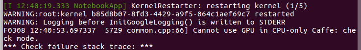
直接将

caffe.set_device(0)

注释掉或删除。因为没有GPU，这条命令只在GPU上运行

继续添加

如果不需要绘制曲线，只需要训练出一个caffemodel, 直接调用solver.solve()就可以了。如果要绘制曲线，就需要把迭代过程中的值

保存下来，因此不能直接调用solver.solve(), 需要迭代。在迭代过程中，每迭代200次测试一次

%%time
niter =4000
test_interval = 200
train_loss = np.zeros(niter)
test_acc = np.zeros(int(np.ceil(niter / test_interval)))

# the main solver loop
for it in range(niter):
    solver.step(1)  # SGD by Caffe
    
    # store the train loss
    train_loss[it] = solver.net.blobs['loss'].data
    solver.test_nets[0].forward(start='conv1')
    
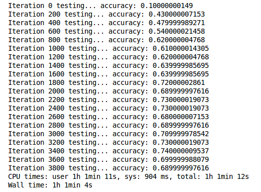
    if it % test_interval == 0:
        acc=solver.test_nets[0].blobs['accuracy'].data
        print 'Iteration', it, 'testing...','accuracy:',acc
        test_acc[it // test_interval] = acc

运行后结果：

绘制train过程中的loss曲线，和测试过程中的accuracy曲线

print test_acc
_, ax1 = plt.subplots()
ax2 = ax1.twinx()
ax1.plot(np.arange(niter), train_loss)
ax2.plot(test_interval * np.arange(len(test_acc)), test_acc, 'r')
ax1.set_xlabel('iteration')
ax1.set_ylabel('train loss')
ax2.set_ylabel('test accuracy')

文章主要参考：http://www.cnblogs.com/denny402/p/5686067.html