vlfeat Gaussian Mixture Models Tutorials

原始的vlfeat 上的Tutorials 代码存在一些错误，在本文中已更正。

This tutorial shows how to estiamte Gaussian mixture model using the VlFeat implementation of the Expectation Maximization (EM) algorithm.

A GMM is a collection of  K Gaussian distribution. Each distribution is called a mode of the GMM and represents a cluster of data points. In computer vision applications, GMM are often used to model dictionaries of visual words. One important application is the computation of Fisher vectors encodings.

(本博客系原创，转载请注明出处：http://blog.csdn.net/xuexiyanjiusheng/article/details/46931695)

Learning a GMM with expectation maximization

Consider a dataset containing 1000 randomly sampled 2D points:

numPoints = 1000 ;
dimension = 2 ;
data = rand(dimension,numPoints) ;

The goal is to fit a GMM to this data. This can be obtained by running the vl_gmm function, implementing the EM algorithm.

numClusters = 30 ;
[means, covariances, priors] = vl_gmm(data, numClusters) ;

Here means, covariances and priors are respectively the means  μk ,diagonal covariance matrices  Σk , and prior probabilities   πk  of the numClusters Gaussian modes.

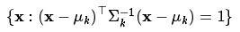
These modes can be visualized on the 2D plane by plotting ellipses corresponding to the equation:

for each of the modes. To this end, we can use the vl_plotframe:

figure ;
hold on ;
plot(data(1,:),data(2,:),'r.') ;
for i=1:numClusters
    %vl_plotframe([means(:,i)' sigmas(1,i) 0 sigmas(2,i)]);
  vl_plotframe([means(:,i)' covariances(1,i) 0 covariances(2,i)]);

end

This results in the figure:

GMM fittting 2D random points.

Diagonal covariance restriction

Note that the ellipses in the previous example are axis alligned. This is a restriction of the vl_gmm implementation that imposes covariance matrices to be diagonal.

This is suitable for most computer vision applications, where estimating a full covariance matrix would be prohebitive due to the relative high dimensionality of the data. For example, when clustering SIFT features, the data has dimension 128, and each full covariance matrix would contain more than 8k parameters.

For this reason, it is sometimes desirable to globally decorrelated the data before learning a GMM mode. This can be obtained by pre-multiplying the data by the inverse of a square root of its covariance.

Initializing a GMM model before running EM

The EM algorithm is a local optimization method, and hence particularly sensitive to the initialization of the model. The simplest way to initiate the GMM is to pick numClusters data points at random as mode means, initialize the individual covariances as the covariance of the data, and assign equa prior probabilities to the modes. This is the default initialization method used by vl_gmm.

Alternatively, a user can specifiy manually the initial paramters of the GMM model by using the custom initalization method. To do so, set the'Initialization' option to 'Custom' and also the options 'InitMeans', 'InitCovariances' and 'IniPriors' to the desired values.

A common approach to obtain an initial value for these parameters is to run KMeans first, as demonstrated in the following code snippet:

numClusters = 30;
numData = 1000;
dimension = 2;
data = rand(dimension,numData);

% Run KMeans to pre-cluster the data
[initMeans, assignments] = vl_kmeans(data, numClusters, ...
    'Algorithm','Lloyd', ...
    'MaxNumIterations',5);

initCovariances = zeros(dimension,numClusters);
initPriors = zeros(1,numClusters);

% Find the initial means, covariances and priors
for i=1:numClusters
    data_k = data(:,assignments==i);
    initPriors(i) = size(data_k,2) / numClusters;

    if size(data_k,1) == 0 || size(data_k,2) == 0
        initCovariances(:,i) = diag(cov(data'));
    else
        initCovariances(:,i) = diag(cov(data_k'));
    end
end

% Run EM starting from the given parameters
[means,covariances,priors,ll,posteriors] = vl_gmm(data, numClusters, ...
    'initialization','custom', ...
    'InitMeans',initMeans, ...
    'InitCovariances',initCovariances, ...
    'InitPriors',initPriors);

The demo scripts vl_demo_gmm_2d_rand, vl_demo_gmm_2d_twist and vl_demo_gmm_3d also produce cute colorized figures such as these:

The figure shows how the estimated gaussian mixture looks like with and without the kmeans initialization.