Sift特征

最新推荐文章于 2024-05-07 10:59:23 发布

机器学习的小学生

最新推荐文章于 2024-05-07 10:59:23 发布

阅读量5.6k

点赞数

分类专栏：面部特征点\face alignment

本文链接：https://blog.csdn.net/raby_gyl/article/details/52607670

版权

面部特征点\face alignment 专栏收录该内容

13 篇文章 0 订阅

订阅专栏

说明：本篇博客只围绕sift描述子展开了学习。对于sift关键点检测涉及的内容并未进行详细的分析和学习。相关内容可参考本篇博客中的参考文献。

Sift特征

Sift特征包含两个部分，一个是关键点（frame或者keypoint），另外一个就是在关键点处的描述子(descriptor,或者Keypoint descriptor)，更确切的说是关键点所在尺度空间的描述子。

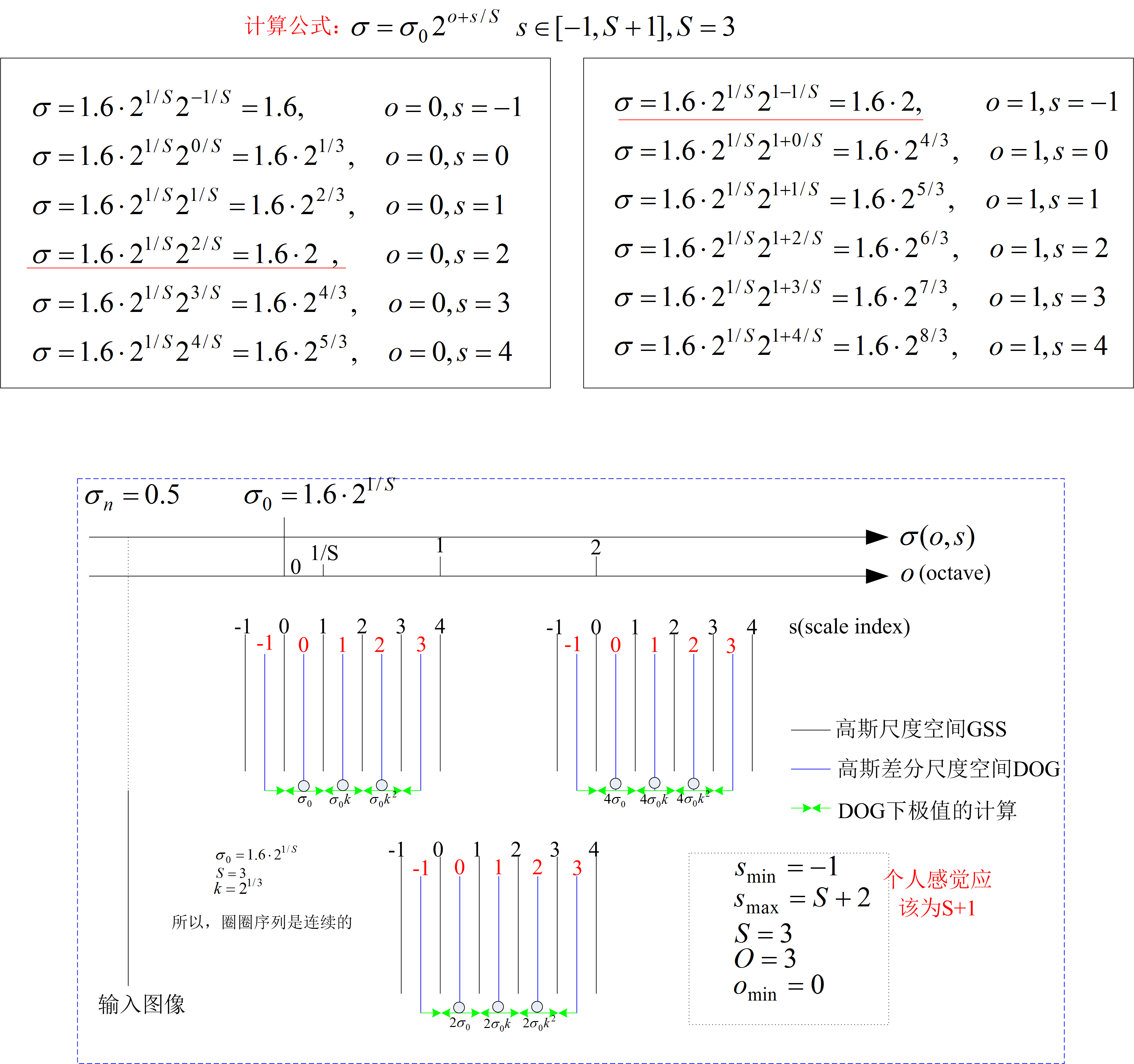
很多文章中给出了两种尺度空间：高斯尺度空间GSS和高斯差分尺度空间DOG。可能会怀疑，到底描述子是在哪个尺度空间计算的？其实采用的是高斯尺度空间。如下图：GSS对图像使用[-1,4]不同尺度的高斯进行平滑得到图像，其索引号[-1,4]指明了不同的尺度，DOG索引号为[-1,3]只是表示与GSS索引号对应的关系，并且图中还给出了”DOG下极值的计算“的索引号，其为GSS的中间三个，即[0,2]。例如，如果我们在”DOG下极值的计算“，发现在其索引号为0尺度有满足条件的关键点，那么该关键点所处的尺度空间就是： $s=0$ 的高斯尺度空间。

在面部特征点的检测中，经常提取Sift特征。这里的Sift特征指的就是Sift描述子，在一个点处提取的Sift特征一般为128维，即4*4*8=128,4*4表示4*4的区域，8表示每个区域统计的方向。

在Vfleat中:frame 表示Keypoint,descriptor 表示Keypoint descriptor

自定义关键点：

vl_sift函数可以自定义关键点，然后计算该关键点处的描述子。

例如我们可以计算关键点在(100,100)，尺度为10,方向为 $-\frac{\pi}{8}$ 的描述子：

fc=[100;100;10;-pi/8];
[f,d]=vl_sift(I,'frames',fc);

我们不指定方向，使用关键点的方向，即将方向参数设置为0，并通过参数’orientations’指定，则：

fc=[100;100;10;0];
[f,d]=vl_sift(I,'frames',fc,'orientations');

也可以将参数fc设置为矩阵的形式，一次计算多个关键点的描述子。特别的，一个关键点可能有多个方向，或者没有方向（图像区域为常数）

问题就来了，这里的尺度是什么？描述子的方向怎么计算的呢？如果方向是指描述子的主方向，那么通过直方图确定主方向时采用的邻域是多大呢？
如上面的函数，我们传入的尺度为10，是使用标准差为 $\sigma=10$ 的高斯对图像进行平滑后，然后进行后面的处理吗？等等一连串的问题，使得我很模糊。
下图给出了高斯尺度示意图，其中左右表格内画红色的下划线的表示（这里我们下表都从0开始）：第1层的第0个图像，是从第0层的第3个图像下采样得到，随后第1层的第1个图像是由第1层的第0个图像再经过高斯标准差为 $\sqrt{\sigma_{(1,0)}^2-\sigma_{(1,-1)}^2}$ 的高斯平滑后得到的，以次类推。。。

这里写图片描述

Vlfeat库的配置：

Vlfeat的源程序使用C语言编写，读起来和使用起来也着实让人费力。由于Vlfeat给出了能够计算给定关键点的描述子的Matlab接口函数。那么我们Matlab入口运行程序进行学习分析。
Vlfeat提供的两个版本：
(1).vlfeat-0.9.20-bin.tar.gz （编译好的二进制文件）
(2).vlfeat-0.9.20 （源文件）

1.下载完vlfeat-0.9.20后，将其解压到当前文件夹，在目录下，有个Makefile.mak文件。使用写字板或者Notepad打开，该文件内给出了需要修改的详细说明，即Customization（定制）部分。

#                                                        Customization
# --------------------------------------------------------------------
# To modify this script to run on your platform it is usually
# sufficient to modify the following variables:
#
# ARCH: Either win32 or win64 [win64]
# DEBUG: Set to yes to ativate debugging [no]
# MATLABROOT: Path to MATLAB
# MSVSVER: Visual Studio version (e.g. 80, 90, 100) [90 for VS 9.0]
# MSVCROOT: Visual C++ location [$(VCInstallDir)].
# WINSDKROOT: Windows SDK location [$(WindowsSdkDir)]
#
# Note that some of these variables depend on the architecture
# (either win32 or win64).

修改截图如下：
这里写图片描述
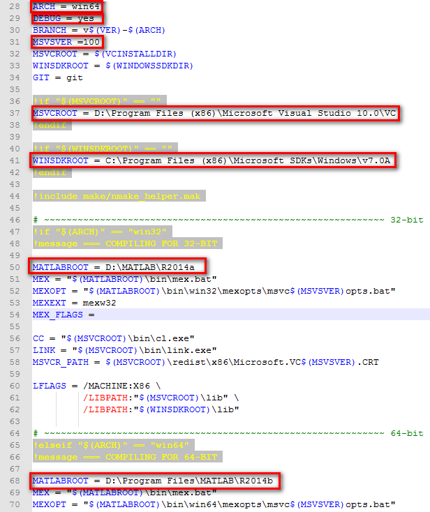
我们电脑上装了两个Matlab，R2014a是32位的，R2014b是64位的。

2.
方法1：双击vlfeat.vcproj打开，进入VS2010界面，点击直到完成后，在左侧的解决方案一栏，对vlfeat进行编译，即build即可。
方法2：在电脑程序目录下，找到Visio Studio Tools找到类似于Visual Studio x64 Win64 命令提示(2010)的工具，点击运行，然后在dos下，将目录切换到vlfeat-0.9.20目录，然后利用nmake命令：

nmake /f Makefile.mak

3.目的：将mex.c文件编译成供Matlab调用的二进制文件。
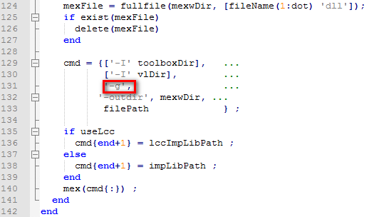
打开Matlab，将工程目录切换到vlfeat-0.9.20\toolbox目录下，首先修改一下vl_compile.m文件，即将mex -o，修改为mex -g，如下：
这里写图片描述

调试Sift源文件

1.打开Matlab，当然首先是要设置好包含路径，主页-设置路径-添加并包含子文件夹，将vlfeat-0.9.20添加进去。我为了省事，一般都是直接将所有的添加进去，你可以选择只需要将toolbox/mex添加到Matlab路径中。然后书写简单的代码：

%clc;clearvars;
% prepare data
imgPath='E:\data\lfw\imgs\Aaron_Eckhart\Aaron_Eckhart_0001.jpg';
bbox=[63 72 126+63 126+72];
landmark=[34 35; 53 38; 41 86; 75 90; 58 93; 59 87 ;72 40 ;94 43; 48 70; 72 72];
nlandmark=10;
isShow=false;
for i=1:nlandmark
    landmark(i,1)=landmark(i,1)+bbox(1);
    landmark(i,2)=landmark(i,2)+bbox(2);
end

if isShow
    figure(1);
    subplot(2,1,1);
    img=imread(imgPath);
    img_gray=rgb2gray(img);
    imshow(img_gray);
    hold on;
    for i=1:nlandmark
        plot(landmark(i,1),landmark(i,2),'.r','markersize',8);
    end
    % for box;
    rmpath('E:\matlabworkplace\headpose_with_block\third_part\vlfeat-0.9.20\toolbox\noprefix');
    plotbox(bbox,'r');
    addpath('E:\matlabworkplace\headpose_with_block\third_part\vlfeat-0.9.20\toolbox\noprefix');
end

% I = vl_impattern('roofs1') ;
% image(I) ;
% I = single(rgb2gray(I)) ;
% [f,d] = vl_sift(I) ;
% perm = randperm(size(f,2)) ;
% sel = perm(1:50) ;
% h1 = vl_plotframe(f(:,sel)) ;
% h2 = vl_plotframe(f(:,sel)) ;
% set(h1,'color','k','linewidth',3) ;
% set(h2,'color','y','linewidth',2) ;

pi=3.1415926;
img=imread(imgPath);
figure(1);
%subplot(1,2,1);
image(img);
img_gray=rgb2gray(img);
I=single(img_gray);
hold on;
ori=[pi/8 2*pi/8 3*pi/8 4*pi/8 5*pi/8 6*pi/8 7*pi/8 pi -pi/8 -2*pi/8];
%scale=[1 2 3 4 5 6 7 8 9 10];
scale=[1.6 1.6 1.6 1.6 1.6 1.6 1.6 1.6 1.6 1.6];
for i=1:10
    plot(landmark(i,1),landmark(i,2),'.r','markersize',16);
    fc=[landmark(i,1);landmark(i,2);scale(i);ori(i)];
    [f,d]=vl_sift(I,'frames',fc);
    h1=vl_plotframe(f(:,1));
    h2=vl_plotframe(f(:,1));
    set(h1,'color','k','linewidth',3);
    set(h2,'color','y','linewidth',2);
    name=num2str(i);
    text(landmark(i,1),landmark(i,2),name);
end
%%上面的代码可以不需要，只需要下面的代码。
figure(2);
img2 = vl_impattern('roofs1') ;
image(img2) ;
img2 = single(rgb2gray(img2)) ;
[f,d] = vl_sift(img2) ;
perm = randperm(size(f,2)) ;
sel = perm(1:50) ;
h1 = vl_plotframe(f(:,sel)) ;
h2 = vl_plotframe(f(:,sel)) ;
set(h1,'color','k','linewidth',3) ;
set(h2,'color','y','linewidth',2) ;
h3 = vl_plotsiftdescriptor(d(:,sel),f(:,sel)) ;
set(h3,'color','g') ;

2.打开VS2010，通过菜单中的文件-打开-文件，将vlfeat-0.9.20\toolbox\sift下的vl_sift.c和vlfeat-0.9.20\vl下的sift.c添加到VS中，然后在两个文件中，设置断点就可以了。
3.在VS2010中设置为断点后，在VS菜单中工具-附加到进程，在可用进程中找到Matlab，然后双击即可。
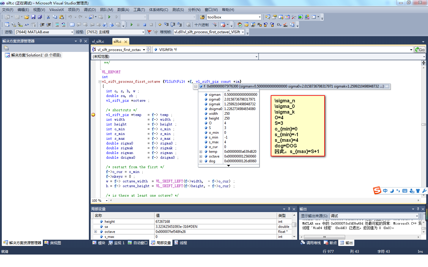
4.运行Matlab程序，会自动跳转到VS2010设置的断点处，通过F5进行断点的切换。如下图：
这里写图片描述

参数说明

公式1：

G (x; σ) = (g σ * I) (x)

$G(x;\sigma)=(g_{\sigma}*I)(x)$
其中

gσ $g_{\sigma}$ 是各向同性高斯核，方差为

σ2I ${\sigma}^2I$ 。
公式2:

σ (o, s) = σ 0 2 o + s / S, o \in o m i n + [0, . . ., O - 1], s \in [0, . . ., S - 1]

$\sigma(o,s)=\sigma_0 2^{o+s/S},o\in o_\mathrm{min}+[0,...,O-1],s\in[0,...,S-1]$
注意这里的

s∈[0,...,S−1] $s\in[0,...,S-1]$ 也着实让人迷惑的，你会在后面看到文章中又有

s∈[smin,smax] $s \in[s_\mathrm{min},s_\mathrm{max}]$ ,其中

smin=−1 $s_\mathrm{min}=-1$ ,

smax=S+1 $s_\mathrm{max}=S+1$

变量	描述
NumOctaves	octaves的数目-O
FirstOctave	第一个octave的索引： $o_\mathrm{min}$ ,octave的索引范围为 $o_\mathrm{min}$ ,…, $o_\mathrm{min}$ +O-1，通常为0或者-1.将 $o_\mathrm{min}$ 设置为-1，就是在计算高斯尺度空间时，将图像长宽扩大一倍的效果。
NumLevels	子层的数量-S
Sigma0	基平滑 Base smoothing
SigmaN	称为预平滑：这是输入图像的预平滑水平。算法假定输入图像实际上不是 $I(x)$ ，而是 $(g_{\sigma_n}*I)(x)$ ,调整计算的依据，通常假定 $\sigma_n$ 是半个像素(0.5)。因此在后面的计算高斯金字塔时，我们想使用初始的 $\sigma_0=1.6$ 进行高斯平滑，但是由于图像假定已经不是纯的 $I$ ，而是进行了 $\sigma_n$ 的平滑，因此，我们只需要在进行 $\sqrt{{\sigma_0}^2-{\sigma_n}^2}$ 的高斯平滑就够了，其等价于原始的纯的I经过方差为 $\sigma_0$ 的高斯平滑。就像别的文章讲的那样，如果初始的o=-1,即将原图像进行了double,即长和宽扩大了两倍，那么此时的 $\sigma_n$ 取1

检测器参数：

SIFT frame（即关键点）是差分尺度空间的局部极值点。这样的点的选择通过下面的参数控制：

变量	描述
Thread	局部极值点阈值，如果局部极值点的 $\|G(x;\sigma)\|$ 小于该阈值，则去掉
EdgeThreshold	局部极值定位阈值，如果局部极值点在一个山谷上，算法丢掉该极值点，因为它太不稳定了。如果极值的得分正比于其陡峭程度，并且得分又小于这个阈值的话，则丢掉该极值点
RemoveBoundaryPoints	边界点的移除，如果这个参数设置为1（即true），太接近图像边界的关键点将被移除。

描述子参数：
SIFT描述子是一个带有权重和插值的直方图，其利用梯度方向和关键点周围的块区域的位置进行计算。描述子有下面的参数：

变量	描述
Magnif	放大因子或者放大倍数m,直方图的每一个空间bin的大小为 $m\sigma$ (单位为像素），其中 $\sigma$ 是该关键点处的尺度,m一般取3.
NumSpatialBins	空间bin的数量，和下面的NumOrientBins参数一起，定义了描述子的扩展和维度。描述子的维度（bins的总数量）等于 $\mathrm{NumSpatialBins}^2×\mathrm{NumOrientBins}$ ,描述子的扩展（即直方图统计区域（块））的半径为 $\mathrm{NumSpatialBins}×m\sigma/2$ ），例如一般为NumSpatialBins=4,NumOrientBins=8，则为448=128，即描述子的维度
NumOrientBins	方向bins的数目

代码的分析

高斯模板

一维高斯:

G (x, σ) = 1 2 π σ 2 - - - - \sqrt e - x 2 2 σ 2

$G(x,\sigma)=\frac{1}{\sqrt{2\pi {\sigma}^2}} e^{\frac{-x^2}{2 {\sigma}^2}}$
二维高斯：

G (x, y, σ I) = G (x, σ) \cdot G (y, σ) = 1 2 π σ 2 - - - - \sqrt e - x 2 2 σ 2 \cdot 1 2 π σ 2 - - - - \sqrt e - y 2 2 σ 2 = 1 2 π σ 2 e - ( x 2 + y 2 ) 2 σ 2

$G(x,y,\sigma I)=G(x,\sigma)\cdot G(y,\sigma)=\frac{1}{\sqrt{2\pi {\sigma}^2}} e^{\frac{-x^2}{2 {\sigma}^2}}\cdot \frac{1}{\sqrt{2\pi {\sigma}^2}} e^{\frac{-y^2}{2 {\sigma}^2}}=\frac{1}{{2\pi {\sigma}^2}} e^{\frac{-({x^2+y^2})}{2 {\sigma}^2}}$

其中 $I$ 是2*2的单位阵。 $x,y$ 具有同样的标准差 $\sigma$ 。
从上面的公式，直观上我们感觉二维高斯卷积操作可以分解为分别经过 $x,y$ 方向的一维操作。这里的“卷积”相当于“相关”。其中 $x,y$ 表示与模板中心的位移。

证明：

G (x, y) * I (x, y) = G (x) * (G (y) * I (x, y))

$G(x,y)*I(x,y)=G(x)*(G(y)*I(x,y))$

G (x, y) * I (x, y) = \int τ \int t G (τ, t) I (τ - x, t - y) d t d τ = \int τ \int t G (τ) G (t) I (τ - x, t - y) d t d τ = \int τ G (τ) (\int t G (t) I (τ - x, t - y) d t) d τ

$\begin{equation} \begin{aligned} G(x,y)*I(x,y) &=\int_{\tau} \int_{t}G(\tau,t)I(\tau-x,t-y)dtd\tau\\ &=\int_{\tau} \int_{t}G(\tau)G(t)I(\tau-x,t-y)dt d\tau\\ &=\int_{\tau} G(\tau)\left (\int_{t}G(t)I(\tau-x,t-y)dt \right) d\tau \end{aligned} \end{equation}$
其中

\int t G (t) I (τ - x, t - y) d t = G (y) * I (τ - x, y)

$\int_{t}G(t)I(\tau-x,t-y)dt =G(y)*I(\tau-x,y)$
而：

\int τ G (τ) (\int t G (t) I (τ - x, t - y) d t) d τ = G (x) * (G (y) * I (τ - (τ - x), y)) = G (x) * G (y) * I (x, y)

$\int_{\tau} G(\tau)\left (\int_{t}G(t)I(\tau-x,t-y)dt \right) d\tau =G(x)*(G(y)*I(\tau-(\tau-x),y))=G(x)*G(y)*I(x,y)$
平滑的高斯模板是多大的呢？即多少个像素呢？其是否与现在使用的高斯标准差（即尺度

σ $\sigma$ ）有关呢？
代码中给出了计算：
高斯模板的宽度=

max(⌈4∗σ⌉,1) $\mathrm{max}(\left \lceil 4*\sigma \right \rceil,1)$ ，这里的宽度是半径，例如对于5*5，则宽度为2，对于7*7，则宽度为3，因此高斯模板的大小为：

2 * m a x (⌈ 4 * σ ⌉, 1) + 1

$2*\mathrm{max}(\left \lceil 4*\sigma \right \rceil,1)+1$

static void
_vl_sift_smooth (VlSiftFilt * self,
                 vl_sift_pix * outputImage,
                 vl_sift_pix * tempImage,
                 vl_sift_pix const * inputImage,
                 vl_size width,
                 vl_size height,
                 double sigma)
{
  /* prepare Gaussian filter */
  if (self->gaussFilterSigma != sigma) {
    vl_uindex j ;
    vl_sift_pix acc = 0 ;//vl_sift_pix即float
    if (self->gaussFilter) vl_free (self->gaussFilter) ;
    self->gaussFilterWidth = VL_MAX(ceil(4.0 * sigma), 1) ;
    self->gaussFilterSigma = sigma ;//$\sigma$
    self->gaussFilter = vl_malloc (sizeof(vl_sift_pix) * (2 * self->gaussFilterWidth + 1)) ;//高斯滤波器,二维滤波可以等价分别x方向一维滤波，然后y方向的一维滤波，或者反过来。

    for (j = 0 ; j < 2 * self->gaussFilterWidth + 1 ; ++j) {
      vl_sift_pix d = ((vl_sift_pix)((signed)j - (signed)self->gaussFilterWidth)) / ((vl_sift_pix)sigma) ;//到高斯模板中心的偏移
      self->gaussFilter[j] = (vl_sift_pix) exp (- 0.5 * (d*d)) ;//这里并不需要乘以\frac{1}{\sqrt{2\pi\sigma}}，因为每一项都有同样的。
      acc += self->gaussFilter[j] ;
    }
    for (j = 0 ; j < 2 * self->gaussFilterWidth + 1 ; ++j) {
      self->gaussFilter[j] /= acc ;//将高斯权重归一化，使其和为1
    }
  }

  if (self->gaussFilterWidth == 0) {
    memcpy (outputImage, inputImage, sizeof(vl_sift_pix) * width * height) ;
    return ;
  }
  //进行一维卷积操作
  vl_imconvcol_vf (tempImage, height,
                   inputImage, width, height, width,
                   self->gaussFilter,
                   - self->gaussFilterWidth, self->gaussFilterWidth,
                   1, VL_PAD_BY_CONTINUITY | VL_TRANSPOSE) ;

  vl_imconvcol_vf (outputImage, width,
                   tempImage, height, width, height,
                   self->gaussFilter,
                   - self->gaussFilterWidth, self->gaussFilterWidth,
                   1, VL_PAD_BY_CONTINUITY | VL_TRANSPOSE) ;
}

例如

尺度 $\sigma=1.6$ ,则进行标准差为 $\sqrt{\sigma^2-\sigma_n^2}=1.5199$ 的高斯平滑，即利用 $G_{1.5199}(x,y)$ 对图像 $I$ 进行平滑，其中高斯模板的大小，通过上面的红色求得为7*7。计算描述子实际窗口的区域的大小为：

3 σ * N u m S p a t i a l B i n s * 2 \sqrt 2

$\frac{3\sigma *\mathrm{NumSpatialBins}*\sqrt 2}{2}$
考虑到像素的加权和插值，因此在上面公式加上1（下面有详解，并可参考下面的空间差值图）。乘以

2√ $\sqrt{2}$ 是考虑到块区域的旋转。变成：

3 σ * ( N u m S p a t i a l B i n s + 1 ) * 2 \sqrt 2

$\frac{3\sigma *(\mathrm{NumSpatialBins}+1)*\sqrt 2}{2}$

附录：
两个高斯函数的卷积仍然为一个高斯函数，满足方差为两个高斯函数之和，即：

σ 21 + σ 22 = σ 23

$\sigma_1^2+\sigma_2^2=\sigma_3^2$
因为二维高斯可以分解为分别进行x方向的一维高斯和y方向的一维高斯。所以这里只推导一维的情况。为了描述的统一和简洁，我们用小写的

g1(x) $g_1(x)$ 来表示一维高斯。
参考： http://blog.csdn.net/liguan843607713/article/details/42215965
一维高斯：

g 1 (x) = 1 2 π - - \sqrt σ 1 e - x 2 2 σ 2 1, g 2 (x) = 1 2 π - - \sqrt σ 2 e - x 2 2 σ 2 2

$g_1(x)=\frac{1}{\sqrt{2\pi}\sigma_1}e^{-\frac{x^2}{2\sigma_1^2}},g_2(x)=\frac{1}{\sqrt{2\pi}\sigma_2}e^{-\frac{x^2}{2\sigma_2^2}}$
我们令

f(x) $f(x)$ 表示两个高斯函数的卷积,即：

f (x) = g 1 (x) * g 2 (x) = \int \infty - \infty g 1 (t) g 2 (x - t) d t = \int \infty - \infty g 1 (x - t) g 2 (t) d t

$\begin{equation} \begin{aligned} f(x)=g_1(x)*g_2(x)&=\int_{-\infty}^{\infty}g_1(t)g_2(x-t)dt \\ &=\int_{-\infty}^{\infty}g_1(x-t)g_2(t)dt \end{aligned} \end{equation}$
我们写出完整的式子：

f (x) 令 a = 1 2 σ 2 1 + 1 2 σ 2 2, b = x σ 2 2, 则 上 式 变 成 为 ： = \int \infty - \infty 1 2 π - - \sqrt σ 1 e - t 2 2 σ 2 1 1 2 π - - \sqrt σ 2 e - ( x - t ) 2 2 σ 2 2 d t = 1 2 π σ 1 σ 2 \int \infty - \infty e - [t 2 2 σ 2 1 + ( x - t ) 2 2 σ 2 2] d t = 1 2 π σ 1 σ 2 \int \infty - \infty e - [(1 2 σ 2 1 + 1 2 σ 2 2) t 2 - (2 x 2 σ 2 2) t + x 2 2 σ 2 2] d t = 1 2 π σ 1 σ 2 e - x 2 2 σ 2 2 \int \infty - \infty e - [(1 2 σ 2 1 + 1 2 σ 2 2) t 2 - (x σ 2 2) t] d t = 1 2 π σ 1 σ 2 e - x 2 2 σ 2 2 \int \infty - \infty e - (a t 2 - b t) d t (公 式 1)

$\begin{equation} \begin{aligned} f(x)&=\int_{-\infty}^{\infty}\frac{1}{\sqrt{2\pi}\sigma_1}e^{-\frac{t^2}{2\sigma_1^2}}\frac{1}{\sqrt{2\pi}\sigma_2}e^{-\frac{(x-t)^2}{2\sigma_2^2}}dt \\ &=\frac{1}{{2\pi}\sigma_1\sigma_2}\int_{-\infty}^{\infty}e^{-\left [\frac{t^2}{2\sigma_1^2}+\frac{(x-t)^2}{2\sigma_2^2}\right]}dt\\ &=\frac{1}{{2\pi}\sigma_1\sigma_2}\int_{-\infty}^{\infty}e^{-\left [ \left( \frac{1}{2\sigma_1^2}+\frac{1}{2\sigma_2^2}\right)t^2-\left (\frac{2x}{2\sigma_2^2}\right)t+\frac{x^2}{2\sigma_2^2}\right]}dt\\ &=\frac{1}{{2\pi}\sigma_1\sigma_2}e^{-\frac{x^2}{2\sigma_2^2}}\int_{-\infty}^{\infty}e^{-\left [ \left( \frac{1}{2\sigma_1^2}+\frac{1}{2\sigma_2^2}\right)t^2-\left (\frac{x}{\sigma_2^2}\right)t\right]}dt\\ 令a= \frac{1}{2\sigma_1^2}+\frac{1}{2\sigma_2^2},b=\frac{x}{\sigma_2^2},则上式变成为：\\ &=\frac{1}{{2\pi}\sigma_1\sigma_2}e^{-\frac{x^2}{2\sigma_2^2}}\int_{-\infty}^{\infty}e^{-\left ( at^2-bt\right)}dt \qquad (公式1)\\ \end{aligned} \end{equation}$

我们发现 $e^{-at^2}$ 可以通过下面的形式计算:

\int \infty - \infty e - x 2 d x = π \sqrt, 其 转 化 为 极 坐 标 形 式 进 行 推 导 （ 略 ） 。

$\begin{equation} \begin{aligned} \int_{-\infty}^{\infty}e^{-x^2}dx=\sqrt{\pi},其转化为极坐标形式进行推导（略）。 \end{aligned} \end{equation}$
而和

ebt $e^{bt}$ 的定积分都没法求解。因此，我们利用变量代换的形式，将

ebt $e^{bt}$ 的形式进行消掉，公式（1）转变为：

f (x) 令 t - b 2 a = τ, 则 上 式 变 成 为 : 将 b 和 a 的 表 达 式 带 入 到 上 式 ： = 1 2 π σ 1 σ 2 e - x 2 2 σ 2 2 \int \infty - \infty e - a (t 2 - b a t + b 2 4 a 2 - b 2 4 a 2) d t = 1 2 π σ 1 σ 2 e - x 2 2 σ 2 2 + b 2 4 a \int \infty - \infty e - a (t - b 2 a) 2 d t = 1 2 π σ 1 σ 2 e - x 2 2 σ 2 2 + b 2 4 a \int \infty - \infty e - a τ 2 d τ = 1 2 π σ 1 σ 2 e - x 2 2 σ 2 2 + b 2 4 a 1 a \sqrt \int \infty - \infty e - (a \sqrt τ) 2 d (a \sqrt τ) = 1 2 π σ 1 σ 2 e - x 2 2 σ 2 2 + b 2 4 a 1 a \sqrt π \sqrt = 1 2 π σ 1 σ 2 e - x 2 2 σ 2 2 + x 2 σ 4 2 4 ( 1 2 σ 2 1 + 1 2 σ 2 2 ) 1 ( 1 2 σ 2 1 + 1 2 σ 2 2 ) - - - - - - - - - - \sqrt π \sqrt = 1 2 π σ 1 σ 2 1 ( 1 2 σ 2 1 + 1 2 σ 2 2 ) - - - - - - - - - - \sqrt π \sqrt \cdot e - x 2 2 σ 2 2 + x 2 σ 4 2 4 ( 1 2 σ 2 1 + 1 2 σ 2 2 ) = 1 2 π ( σ 2 1 + σ 2 2 ) - - - - - - - - - - \sqrt \cdot e - x 2 2 ( σ 2 1 + σ 2 2 )

$\begin{equation} \begin{aligned} f(x)&=\frac{1}{{2\pi}\sigma_1\sigma_2}e^{-\frac{x^2}{2\sigma_2^2}}\int_{-\infty}^{\infty}e^{-a\left (t^2-\frac{b}{a}t+\frac{b^2}{4a^2}-\frac{b^2}{4a^2}\right)}dt\\ &=\frac{1}{{2\pi}\sigma_1\sigma_2}e^{-\frac{x^2}{2\sigma_2^2}+\frac{b^2}{4a}}\int_{-\infty}^{\infty}e^{-a\left (t-\frac{b}{2a}\right)^2}dt \\ 令t-\frac{b}{2a}=\tau,则上式变成为:\\ &=\frac{1}{{2\pi}\sigma_1\sigma_2}e^{-\frac{x^2}{2\sigma_2^2}+\frac{b^2}{4a}}\int_{-\infty}^{\infty}e^{-a \tau^2}d\tau\\ &=\frac{1}{{2\pi}\sigma_1\sigma_2}e^{-\frac{x^2}{2\sigma_2^2}+\frac{b^2}{4a}} \frac{1}{\sqrt{a}}\int_{-\infty}^{\infty}e^{-(\sqrt{a} \tau)^2}d(\sqrt{a}\tau)\\ &=\frac{1}{{2\pi}\sigma_1\sigma_2}e^{-\frac{x^2}{2\sigma_2^2}+\frac{b^2}{4a}} \frac{1}{\sqrt{a}}\sqrt{\pi}\\ 将b和a的表达式带入到上式：\\ &=\frac{1}{{2\pi}\sigma_1\sigma_2}e^{-\frac{x^2}{2\sigma_2^2}+\frac{\frac{x^2}{\sigma_2^4}}{4(\frac{1}{2\sigma_1^2}+\frac{1}{2\sigma_2^2})}} \frac{1}{\sqrt{(\frac{1}{2\sigma_1^2}+\frac{1}{2\sigma_2^2})}}\sqrt{\pi}\\ &=\frac{1}{{2\pi}\sigma_1\sigma_2}\frac{1}{\sqrt{(\frac{1}{2\sigma_1^2}+\frac{1}{2\sigma_2^2})}}\sqrt{\pi}\cdot e^{-\frac{x^2}{2\sigma_2^2}+\frac{\frac{x^2}{\sigma_2^4}}{4(\frac{1}{2\sigma_1^2}+\frac{1}{2\sigma_2^2})}} \\ &=\frac{1}{\sqrt{2\pi(\sigma_1^2+\sigma_2^2)}}\cdot e^{-\frac{x^2}{2(\sigma_1^2+\sigma_2^2)}} \end{aligned} \end{equation}$

上面是一维连续高斯的卷积的证明。因此在取高斯窗口大小时采用了:

2 * m a x (⌈ 4 * σ ⌉, 1) + 1

$2*\mathrm{max}(\left \lceil 4*\sigma \right \rceil,1)+1$
就是为了近似的满足上面卷积的要求。即高斯积分的取值范围为(

−∞,+∞ $-\infty,+\infty$ ),即涵盖了高斯的所有取值。而满足上面的大小的窗口能够涵盖高斯的主要取值，所以在离散的空间，经过

σ2 $\sigma_2$ 高斯平滑，近似的等价于先经过

σ1 $\sigma_1$ 的高斯平滑，在经过

σ22−σ21−−−−−−−√ $\sqrt{\sigma_2^2-\sigma_1^2}$ 的高斯平滑（注意这里的

σ2>σ1 $\sigma_2>\sigma_1$ ）。

sift描述子的计算

这里写图片描述
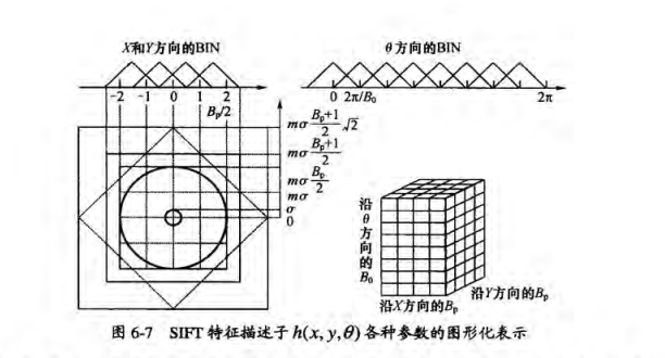
上面的图片来至于：《图像局部不变性特征与描述》，其很好的描述了当前图像所在的尺度和实际像素大小的关系。 $B_p$ 就是上面描述的NumSpatialBins， $m=3$ :

σ 表 示 当 前 描 述 子 所 在 的 尺 度 m σ 表 示 一 个 空 间 bin 的 实 际 像 素 大 小 m σ B p 2 表 示 4*4 空 间 的 半 径 m σ B p + 1 2 考 虑 到 像 素 的 加 权 和 插 值 ， 在 x(或 y) 的 正 负 方 向 扩 展 了 半 个 bin m σ B p + 1 2 2 \sqrt 考 虑 到 图 像 的 旋 转

$\begin{equation} \begin{aligned} \sigma \text{表示当前描述子所在的尺度}\\ m\sigma \text{表示一个空间bin的实际像素大小}\\ m \sigma \frac{B_p}{2} \text{表示4*4空间的半径} \\ m \sigma \frac{B_p+1}{2} \text{考虑到像素的加权和插值，在x(或y)的正负方向扩展了半个bin}\\ m \sigma \frac{B_p+1}{2}{\sqrt{2}} \text{考虑到图像的旋转} \end{aligned} \end{equation}$
下面是VLFeat中描述子计算的代码：

Since weighting and interpolation of pixel is used, the support extends by another half bin.
因为使用了像素的加权和插值，支撑范围扩展了半个bin的像素大小。

下图描述了两种度量单位：1 bin为单位，以及像素单位。1bin= $m \sigma$ ,其中在计算插值时，采用的像素空间为连续的取值。

空间插值：
下图右侧给出了空间方向的插值，其中大小为4*4的空间bin,图中长度的度量方式均是采用1个bin为单位。黄色的点表示当前的像素点，都带有：空间位置，梯度和梯度方向属性，其有4个邻域，其中绿色的点表示每个bin的中心，灰色的点不在bin的范围内。
方向插值：
下图，左侧给出了一个空间bin中的方向的直方图统计（采用梯度幅值进行了加权，看箭头），其中170表示当前某个像素处的梯度方向，其介于157.5和202.5（分别对应于每个bin的中心）之间，那么该像素的梯度在这两个方向bin上的加权分别为w1和w2,w1=(170-157.5)/45,w2=1-w1，其中45为bin的宽度。即将360分成8个bin，每个bin的宽度为45.

对于一个像素（即当前关键点所在的尺度图像中的一个像素），其空间位置确定了其有4个邻域，其方向确定了其有2个方向的邻域。因此共4*2=8个邻域。即利用该像素的梯度对4个相邻空间bin的每两个方向bin进行加权。

有兴趣的话，可以将空间插值和方差插值画在一起，即画在一个三维图中。

这里写图片描述
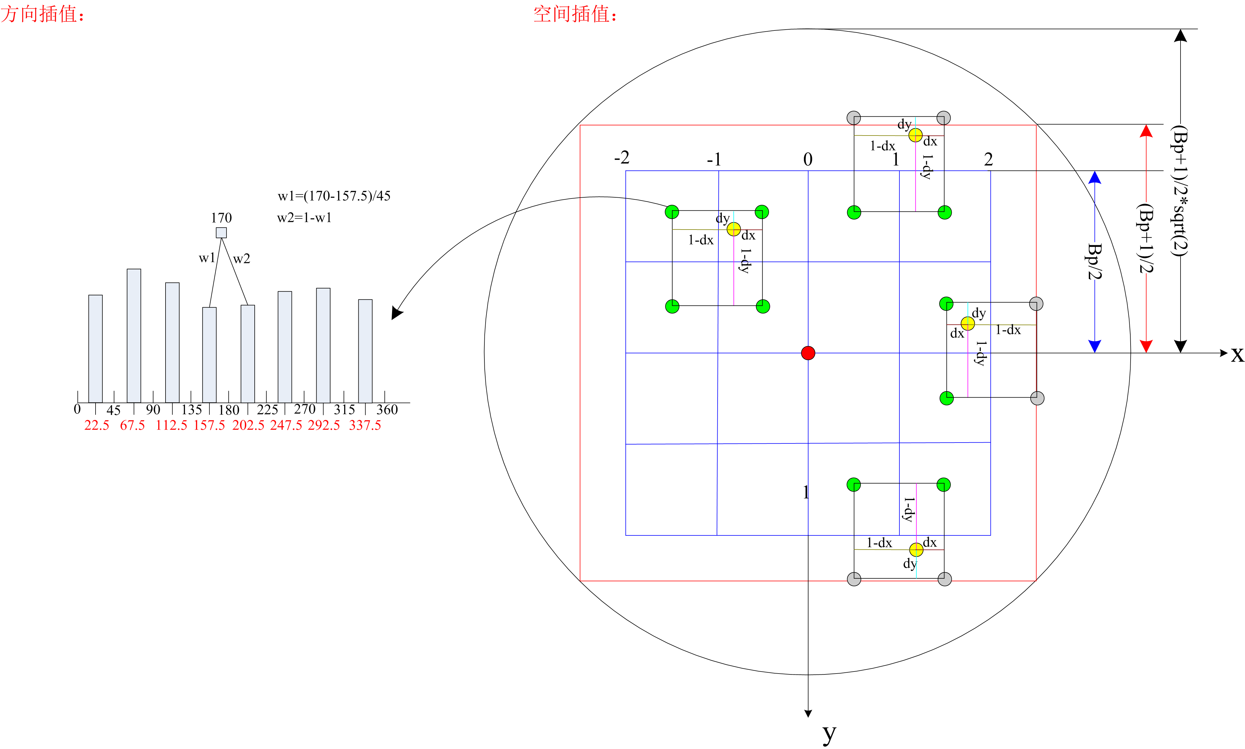
上图，空间插值图有误，下图为修改后

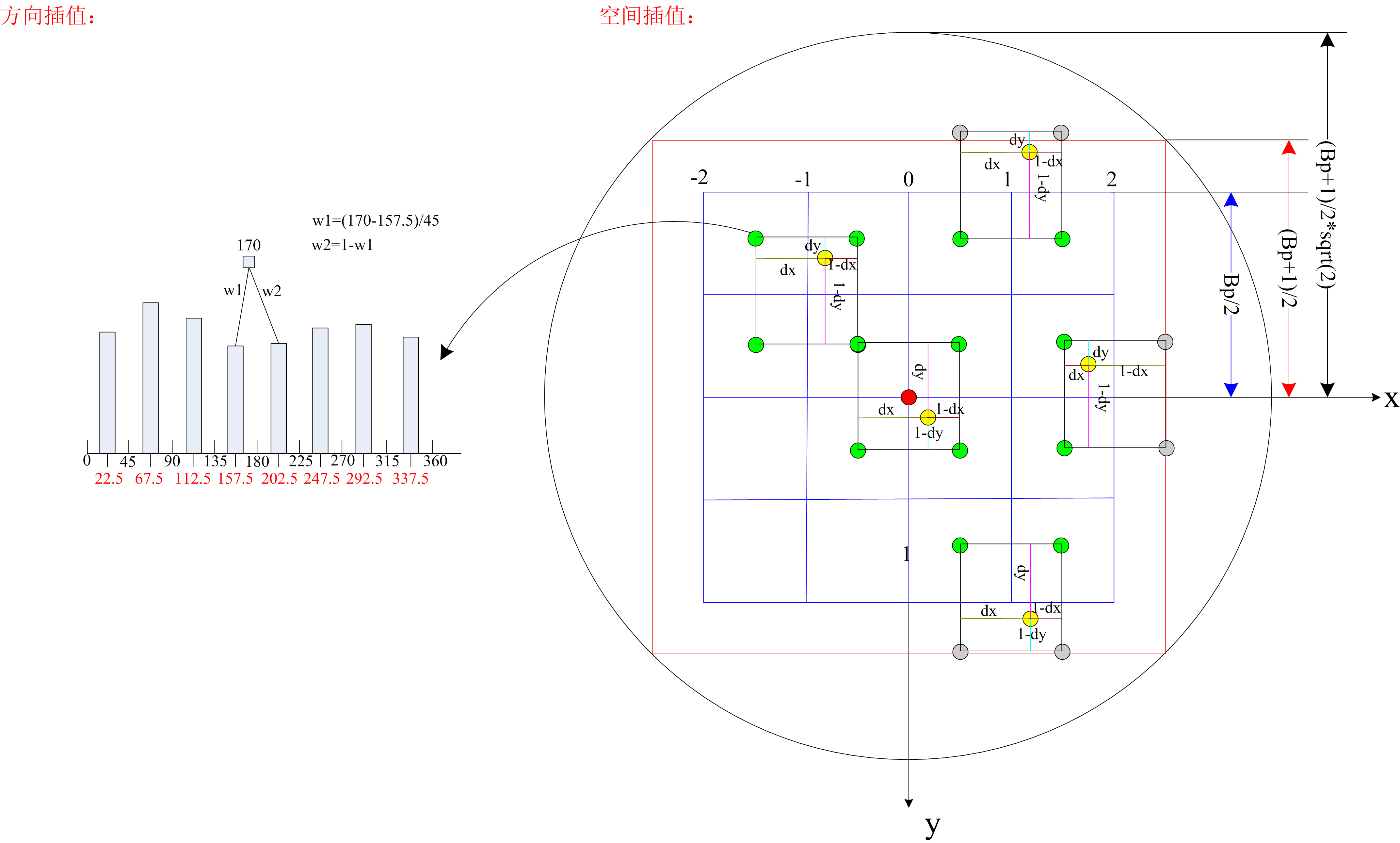
其中dx,dy是相对于黄色点左上角中心（绿色）的距离。

VL_EXPORT
void
vl_sift_calc_keypoint_descriptor (VlSiftFilt *f,
                                  vl_sift_pix *descr,
                                  VlSiftKeypoint const* k,
                                  double angle0)
{
  /*
     The SIFT descriptor is a three dimensional histogram of the
     position and orientation of the gradient.  There are NBP bins for
     each spatial dimension and NBO bins for the orientation dimension,
     for a total of NBP x NBP x NBO bins.

     The support of each spatial bin has an extension of SBP = 3sigma
     pixels, where sigma is the scale of the keypoint.  Thus all the
     bins together have a support SBP x NBP pixels wide. Since
     weighting and interpolation of pixel is used, the support extends
     by another half bin. Therefore, the support is a square window of
     SBP x (NBP + 1) pixels. Finally, since the patch can be
     arbitrarily rotated, we need to consider a window 2W += sqrt(2) x
     SBP x (NBP + 1) pixels wide.
  */

  double const magnif      = f-> magnif ;//3，放大倍数m

  double       xper        = pow (2.0, f->o_cur) ;//步长，针对原图像为250,250的话，如果当前的octave是0，则步长为1，如果octave=1,则步长为2,就是遍历“原图像大小”（不是原图像）的步长

  int          w           = f-> octave_width ;//250
  int          h           = f-> octave_height ;//250
  int const    xo          = 2 ;         /* x-stride *///其将梯度和方向封装在一个数组中，两两间隔，所以步长为2
  int const    yo          = 2 * w ;     /* y-stride */
  int const    so          = 2 * w * h ; /* s-stride *///遍历下一个高斯尺度图像s的步长
  double       x           = k-> x     / xper ;//关键点的位置
  double       y           = k-> y     / xper ;
  double       sigma       = k-> sigma / xper ;//当前的高斯尺度图像对应的尺度，我设置的参数为1.6（针对已知关键点，求描述子的情况）

  int          xi          = (int) (x + 0.5) ;
  int          yi          = (int) (y + 0.5) ;
  int          si          = k-> is ;//有可能是高斯差分对应的索引

  double const st0         = sin (angle0) ;//pi/2-传入的角度pi/8,这里的angle0应该是夹角。
  double const ct0         = cos (angle0) ;
  double const SBP         = magnif * sigma + VL_EPSILON_D ;//m*\sigma 即1个bin的像素大小
  int    const W           = floor
    (sqrt(2.0) * SBP * (NBP + 1) / 2.0 + 0.5) ;//窗口的半径，这里为17，即$\sigma \frac{B_p+1}{2}{\sqrt{2}$,也就是图中外接圆的半径

  int const binto = 1 ;          /* bin theta-stride *///存储的方向bin步长
  int const binyo = NBO * NBP ;  /* bin y-stride *///8*4
  int const binxo = NBO ;        /* bin x-stride *///8

  int bin, dxi, dyi ;
  vl_sift_pix const *pt ;
  vl_sift_pix       *dpt ;

  /* check bounds *///检测边界
  if(k->o  != f->o_cur        ||
     xi    <  0               ||
     xi    >= w               ||
     yi    <  0               ||
     yi    >= h -    1        ||
     si    <  f->s_min + 1    || //0<=si<=2
     si    >  f->s_max - 2     )
    return ;

  /* synchronize gradient buffer *///计算当前octave下，关键点所在的三个尺度(s0,s1,s2)图像上的梯度。问题来了，梯度的计算不是在旋转到主方向在计算吗？
  update_gradient (f) ;

  /* VL_PRINTF("W = %d ; magnif = %g ; SBP = %g\n", W,magnif,SBP) ; */

  /* clear descriptor */
  memset (descr, 0, sizeof(vl_sift_pix) * NBO*NBP*NBP) ;//为描述子分配空间，大小为8*4*4=128，descr描述子的首地址

  /* Center the scale space and the descriptor on the current keypoint.//
   * Note that dpt is pointing to the bin of center (SBP/2,SBP/2,0).
   */
  pt  = f->grad + xi*xo + yi*yo + (si - f->s_min - 1)*so ;//指向关键点处梯度的指针
  dpt = descr + (NBP/2) * binyo + (NBP/2) * binxo ;//指向了描述子的中心，（即直方图的统计中心）binyo表示一行空间bin包括了方向bin，即y_0_即4*8。

#undef atd //at已知dbinx,dbiny,dbint定位其元素值在数组中的位置
#define atd(dbinx,dbiny,dbint) *(dpt + (dbint)*binto + (dbiny)*binyo + (dbinx)*binxo)

  /*
   * Process pixels in the intersection of the image rectangle
   * (1,1)-(M-1,N-1) and the keypoint bounding box.
   */
   //处理边框[-17 17]中的每一个像素
  for(dyi =  VL_MAX (- W, 1 - yi    ) ;
      dyi <= VL_MIN (+ W, h - yi - 2) ; ++ dyi) {

    for(dxi =  VL_MAX (- W, 1 - xi    ) ;
        dxi <= VL_MIN (+ W, w - xi - 2) ; ++ dxi) {

      /* retrieve *///pt指向了关键点处的梯度指针
      vl_sift_pix mod   = *( pt + dxi*xo + dyi*yo + 0 ) ;//梯度
      vl_sift_pix angle = *( pt + dxi*xo + dyi*yo + 1 ) ;//角度//梯度和角度存储在同一个数组中，相互间隔，所以+1就可以遍历到
      vl_sift_pix theta = vl_mod_2pi_f (angle - angle0) ;//如果angle0为主方向的化，angle-angle0相当于该像素的方向与主方向之间的夹角或者差值

      /* fractional displacement */ 关键点离散像素位置和精确位置的偏移
      vl_sift_pix dx = xi + dxi - x;
      vl_sift_pix dy = yi + dyi - y;

      /* get the displacement normalized w.r.t. the keypoint,关于方向和扩展进行标准化，即除以SBP，表示转换为以1bin为单位，即转换到1bin为单位的衡量空间,方向：theta/(2pi/8),角度也是以45bin长为单位，只是换成了弧度制。
         orientation and extension */
      vl_sift_pix nx = ( ct0 * dx + st0 * dy) / SBP ;
      vl_sift_pix ny = (-st0 * dx + ct0 * dy) / SBP ;
      vl_sift_pix nt = NBO * theta / (2 * VL_PI) ;

      /* Get the Gaussian weight of the sample. The Gaussian window
       * has a standard deviation equal to NBP/2. Note that dx and dy
       * are in the normalized frame, so that -NBP/2 <= dx <=
       * NBP/2. */
      vl_sift_pix const wsigma = f->windowSize ;//2,即NBP的一半
      vl_sift_pix win = fast_expn
        ((nx*nx + ny*ny)/(2.0 * wsigma * wsigma)) ;//高斯加权，采用的是标准化到1bin为单位的空间，

      /* The sample will be distributed in 8 adjacent bins.
      //以空间插值图中最左边的黄色像素为例，其大约的位置为(nx,ny)=(-0.75,-1.35), theta=pi/4,nt=0.617那么
      //binx=floor(-0.75-0.5)=-2;左上角的点
      //biny=floor(-1.35-0.5)=-2;左上角的点，
      //bint=1;弧度
      //rbinx=-0.75-(-2+0.5)=-0.75+1.5=0.75;//其中(-2+0.5)定位(-2,-2)对应的bin的中心的x坐标。-0.75-(-2+0.5)表示黄色的点的x坐标到bin的中心点的x坐标之间的距离。
      //rbiny=-1.35-(-2+0.5)=-1.35+0.5=0.15;//同上，(-2+0.5)定位(-2,-2)对应的bin的中心的y坐标，-1.35-(-2+0.5)表示黄色的点的y坐标到bin的中心点的y坐标的距离。
      //rbint=0.617-1=0.383
      //我们知道黄色点所在的bin的中心（蓝色点）的坐标为：(-0.5,-1.5)，则dx=0.25,dy=0.15.
         We start from the ``lower-left'' bin. */ 
      int         binx = (int)vl_floor_f (nx - 0.5) ;
      int         biny = (int)vl_floor_f (ny - 0.5) ;
      int         bint = (int)vl_floor_f (nt) ;
      vl_sift_pix rbinx = nx - (binx + 0.5) ;
      vl_sift_pix rbiny = ny - (biny + 0.5) ;
      vl_sift_pix rbint = nt - bint ;
      int         dbinx ;
      int         dbiny ;
      int         dbint ;

      /* Distribute the current sample into the 8 adjacent bins*/
      //例如空间插值图中，最左边的黄色点，其binx指向(-2,-2)所在的左上角的bin，那么binx+dbinx=binx+0,则表示还是指向该bin,而binx+dbinx=binx+1,则表示指向的黄色点所在的bin，对于binxy同理。再比如，最右边的黄色的点，计算的binx值应该是它所在的bin...
      for(dbinx = 0 ; dbinx < 2 ; ++dbinx) {
        for(dbiny = 0 ; dbiny < 2 ; ++dbiny) {
          for(dbint = 0 ; dbint < 2 ; ++dbint) {

            if (binx + dbinx >= - (NBP/2) &&
                binx + dbinx <    (NBP/2) &&
                biny + dbiny >= - (NBP/2) &&
                biny + dbiny <    (NBP/2) ) {
              vl_sift_pix weight = win
                * mod
                * vl_abs_f (1 - dbinx - rbinx)
                * vl_abs_f (1 - dbiny - rbiny)
                * vl_abs_f (1 - dbint - rbint) ;

              atd(binx+dbinx, biny+dbiny, (bint+dbint) % NBO) += weight ;//数组下标的离散。例如a[-2]就不是当前指针a，向前移动两步。
            }
          }
        }
      }
    }
  }

  /* Standard SIFT descriptors are normalized, truncated and normalized again */
  if(1) {

    /* Normalize the histogram to L2 unit length. */
    //descr描述子的首地址，descr+NBO*NBP*NBP描述子的尾地址
    vl_sift_pix norm = normalize_histogram (descr, descr + NBO*NBP*NBP) ;

    /* Set the descriptor to zero if it is lower than our norm_threshold *///我们这里norma_thresh=0,norm为258
    if(f-> norm_thresh && norm < f-> norm_thresh) {
        for(bin = 0; bin < NBO*NBP*NBP ; ++ bin)
            descr [bin] = 0;
    }
    else {

      /* Truncate at 0.2. */
      //不能超过0.2
      for(bin = 0; bin < NBO*NBP*NBP ; ++ bin) {
        if (descr [bin] > 0.2) descr [bin] = 0.2;
      }

      /* Normalize again. */再次进行标准化
      normalize_histogram (descr, descr + NBO*NBP*NBP) ;
    }
  }

}

上面的代码给出加权的计算公式：

vl_sift_pix weight = win
                * mod
                * vl_abs_f (1 - dbinx - rbinx)
                * vl_abs_f (1 - dbiny - rbiny)
                * vl_abs_f (1 - dbint - rbint) ;

其中：

w i n = m o d = r b i n x, = d b i n x, d b i n y \in e - ( x 2 + y 2 ) 2 σ 2 w, σ w = B p / 2 = 2 梯 度 幅 值 d x, r b i n y = d y, 其 中 0 \leq d x \leq 0.5, 0 \leq d y \leq 0.5 ， 单 位 为 1 b i n {0, 1} ， 当 0 时 为 : 1 - d x, 当 1 时 为 : d x, 以 此 类 推 . . .

$\begin{equation} \begin{aligned} \mathrm{win}=&e^{-{\frac{(x^2+y^2)}{2\sigma_w^2}}},\sigma_w=Bp/2=2\\ \mathrm{mod}=&梯度幅值\\ \mathrm{rbinx},=&dx,\mathrm{rbiny}=dy,其中0 \leq dx \leq 0.5,0 \leq dy \leq 0.5，单位为1bin\\ \mathrm{dbinx},\mathrm{dbiny}\in & \{0,1\}，当0时为:1-dx,当1时为:dx,以此类推... \end{aligned} \end{equation}$
所以最后的公式为(为了书写的美观，将

dx $dx$ 写为

dx $d_x$ ，

dy,do $dy,do$ 类似)：

w = | g r a d (I σ (x 0, y 0) | \cdot e - ( x 2 + y 2 ) 2 σ 2 w \cdot (1 - d x) 1 - i d i x \cdot (1 - d y) 1 - j d j y \cdot (1 - d o) 1 - k d k o

$\begin{equation} \begin{aligned} \mathrm{w}=|grad(I_{\sigma}(x_0,y_0)|\cdot & e^{-\frac{(x^2+y^2)}{2\sigma_w^2}}\cdot (1-d_x)^{1-i} d_x^i \cdot(1-d_y)^{1-j}d_y^j \cdot(1-d_o)^{1-k} d_o^k \end{aligned} \end{equation}$
其中:

i,j,k∈{0,1},σ $i,j,k \in \{0,1\},\sigma$ 是当前关键点所在的图像尺度。

x0,y0 $x_0,y_0$ 的单位像素;x,y的单位为1bin(空间bin,范围为[-2,2]，x轴方向,长度为4,y轴方向长度为4，1bin=

3σ $3\sigma$ 像素；

dx,dy $d_x,d_y$ 的单位也是1bin；

do $d_o$ 的单位为1bin（但是是方向bin，bin的范围为[0,8],长度为8，1bin=

2π8=0.25π弧度 $\frac{2\pi}{8}=0.25\pi弧度$ ）。从

x0.y0 $x_0.y_0$ 到

x,y $x,y$ 通过仿射映射和坐标单位换算得到。

VLFeat代码中给出图像旋转后的坐标的计算公式为:

(x' y') = (c o s θ - s i n θ s i n θ c o s θ) (x y) (x, y \in [- r, r])

$\begin{equation} \begin{pmatrix} x'\\ y' \end{pmatrix}=\begin{pmatrix} cos \theta & sin \theta\\ -sin \theta& cos \theta \end{pmatrix} \begin{pmatrix} x\\ y \end{pmatrix}(x,y \in [-r,r]) \end{equation}$
D.Lowe’s sift实现中的计算公式：

(x' y') = (c o s θ s i n θ - s i n θ c o s θ) (x y) (x, y \in [- r, r])

$\begin{equation} \begin{pmatrix} x'\\ y' \end{pmatrix}=\begin{pmatrix} cos \theta & -sin \theta\\ sin \theta& cos \theta \end{pmatrix} \begin{pmatrix} x\\ y \end{pmatrix}(x,y \in [-r,r]) \end{equation}$
之所有会出现上面的差别，是因为选用了不同的坐标系和角度的旋转规则：
下图给出VLFeat实现的约定规则和D.Lowes实现的约定规则：
这里写图片描述

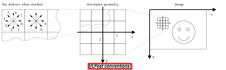
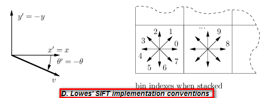
其中VLFeat的代码中，对于输入主方向，例如为 $-\pi/8$ ,其进行了下面的操作：

 angles [0] = VL_PI / 2 - ikeys [4 * i + 3] ;%ikeys[4*i+3]=-pi/8

即：

θ 0 = π 2 - (- π 8)

$\theta_0=\frac{\pi}{2}-(-\frac{\pi}{8})$
下图给出了详细操作的解释：
这里写图片描述

坐标的虚线框内描述了理论上的计算过程，右边虚线框内描述了实际的计算过程，因为Matlab矩阵的存储方式是按列存储的，而c是按行存储的，所以在C中处理的图像其实是实际图像的转置。

sift描述子主方向的计算

这里给出了代码：

VL_EXPORT
int
vl_sift_calc_keypoint_orientations (VlSiftFilt *f,
                                    double angles [4],
                                    VlSiftKeypoint const *k)
{
  double const winf   = 1.5 ;
  double       xper   = pow (2.0, f->o_cur) ;

  int          w      = f-> octave_width ;
  int          h      = f-> octave_height ;
  int const    xo     = 2 ;         /* x-stride */
  int const    yo     = 2 * w ;     /* y-stride */
  int const    so     = 2 * w * h ; /* s-stride */
  double       x      = k-> x     / xper ;
  double       y      = k-> y     / xper ;
  double       sigma  = k-> sigma / xper ;

  int          xi     = (int) (x + 0.5) ;
  int          yi     = (int) (y + 0.5) ;
  int          si     = k-> is ;

  double const sigmaw = winf * sigma ;
  int          W      = VL_MAX(floor (3.0 * sigmaw), 1) ;

  int          nangles= 0 ;

  enum {nbins = 36} ;

  double hist [nbins], maxh ;
  vl_sift_pix const * pt ;
  int xs, ys, iter, i ;

  /* skip if the keypoint octave is not current */
  if(k->o != f->o_cur)
    return 0 ;

  /* skip the keypoint if it is out of bounds */
  if(xi < 0            ||
     xi > w - 1        ||
     yi < 0            ||
     yi > h - 1        ||
     si < f->s_min + 1 ||
     si > f->s_max - 2  ) {
    return 0 ;
  }

  /* make gradient up to date */
  update_gradient (f) ;

  /* clear histogram */
  memset (hist, 0, sizeof(double) * nbins) ;

  /* compute orientation histogram */
  pt = f-> grad + xo*xi + yo*yi + so*(si - f->s_min - 1) ;

#undef  at
#define at(dx,dy) (*(pt + xo * (dx) + yo * (dy)))

  for(ys  =  VL_MAX (- W,       - yi) ;
      ys <=  VL_MIN (+ W, h - 1 - yi) ; ++ys) {

    for(xs  = VL_MAX (- W,       - xi) ;
        xs <= VL_MIN (+ W, w - 1 - xi) ; ++xs) {


      double dx = (double)(xi + xs) - x;
      double dy = (double)(yi + ys) - y;
      double r2 = dx*dx + dy*dy ;
      double wgt, mod, ang, fbin ;

      /* limit to a circular window */
      if (r2 >= W*W + 0.6) continue ;

      wgt  = fast_expn (r2 / (2*sigmaw*sigmaw)) ;
      mod  = *(pt + xs*xo + ys*yo    ) ;
      ang  = *(pt + xs*xo + ys*yo + 1) ;
      fbin = nbins * ang / (2 * VL_PI) ;

#if defined(VL_SIFT_BILINEAR_ORIENTATIONS)
      {
        int bin = (int) vl_floor_d (fbin - 0.5) ;
        double rbin = fbin - bin - 0.5 ;
        hist [(bin + nbins) % nbins] += (1 - rbin) * mod * wgt ;
        hist [(bin + 1    ) % nbins] += (    rbin) * mod * wgt ;
      }
#else
      {
        int    bin  = vl_floor_d (fbin) ;
        bin = vl_floor_d (nbins * ang / (2*VL_PI)) ;
        hist [(bin) % nbins] += mod * wgt ;
      }
#endif

    } /* for xs */
  } /* for ys */

  /* smooth histogram */
  for (iter = 0; iter < 6; iter ++) {
    double prev  = hist [nbins - 1] ;
    double first = hist [0] ;
    int i ;
    for (i = 0; i < nbins - 1; i++) {
      double newh = (prev + hist[i] + hist[(i+1) % nbins]) / 3.0;
      prev = hist[i] ;
      hist[i] = newh ;
    }
    hist[i] = (prev + hist[i] + first) / 3.0 ;
  }

  /* find the histogram maximum */
  maxh = 0 ;
  for (i = 0 ; i < nbins ; ++i)
    maxh = VL_MAX (maxh, hist [i]) ;

  /* find peaks within 80% from max */
  nangles = 0 ;
  for(i = 0 ; i < nbins ; ++i) {
    double h0 = hist [i] ;
    double hm = hist [(i - 1 + nbins) % nbins] ;
    double hp = hist [(i + 1 + nbins) % nbins] ;

    /* is this a peak? */
    if (h0 > 0.8*maxh && h0 > hm && h0 > hp) {

      /* quadratic interpolation */
      double di = - 0.5 * (hp - hm) / (hp + hm - 2 * h0) ;
      double th = 2 * VL_PI * (i + di + 0.5) / nbins ;
      angles [ nangles++ ] = th ;
      if( nangles == 4 )
        goto enough_angles ;
    }
  }
 enough_angles:
  return nangles ;
}

计算描述子方向的窗口大小为: $w=\max(\left \lfloor3*(\mathrm{win}_f*\sigma)\right \rfloor,1)$ ，其中 $\mathrm{win}_f=1.5，\sigma$ 为当前关键点所在的尺度，本例中w=7,即 $\sigma$ 取1.6。其将360度的方向划成了36个bin(为了确定更精确的方向）。这里是为了计算主方向，在尺度图像上进行梯度，而不需要仿射变换。

高斯金字塔图像

在Vlfeat的vl_sift.cpp中（为了使用opencv,mexopencv,我们将其改为了cpp文件）中添加如下的代码，输出保存高斯图像金字塔。

      if (first) {
        err   = vl_sift_process_first_octave (filt, data) ;
        //add my code,out[2]对图像进行输出
        int smax=4;
        int smin=-1;
        int ns=smax-smin+1;
        vl_sift_pix *oct0 = filt->octave ;
        int o=vl_sift_get_octave_index (filt);
        Mat mat0(M*N,ns,CV_8UC1);
        for(int k=0;k<ns;k++)
        {
            int st=k*M*N;
            for(int jj=0;jj<N;jj++)//N表示列数
                for(int ii=0;ii<M;ii++)//M表示行数
                    mat0.at<uchar>(ii+jj*N,k)=(uchar)oct0[ii+jj*N+st];
        }
        out[o+2]=MxArray(mat0);
        first = 0 ;
      } else {
        err   = vl_sift_process_next_octave  (filt) ;
        //add my code,out[2]对图像进行输出
        int smax=4;
        int smin=-1;
        int ns=smax-smin+1;
        vl_sift_pix *oct0 = filt->octave ;
        int o=vl_sift_get_octave_index (filt);
        int m=M/(pow(2.0,o));
        int n=N/(pow(2.0,o));
        Mat mat0(m*n,ns,CV_8UC1);
        for(int k=0;k<ns;k++)
        {
            int st=k*m*n;
            for(int jj=0;jj<n;jj++)//N表示列数
                for(int ii=0;ii<m;ii++)//M表示行数
                    mat0.at<uchar>(ii+jj*n,k)=(uchar)oct0[ii+jj*n+st];
        }
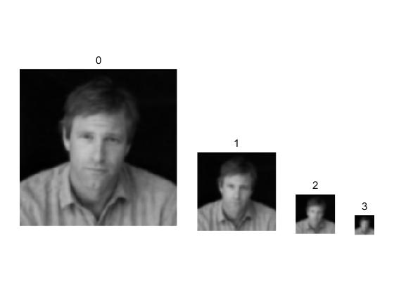
        out[o+2]=MxArray(mat0);

      }

下图给出了，4个octave的第一个s的图像：
这里写图片描述
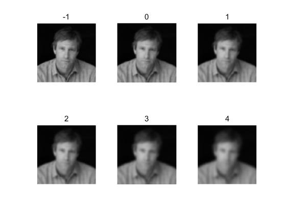
下图给出了第一个octave下的6个尺度图像：

VLFeat中计算给定关键点的描述子时间测试

clearvars;close all;
imgPath='E:\data\lfw\imgs\Aaron_Eckhart\Aaron_Eckhart_0001.jpg';
bbox=[63 72 126+63 126+72];
landmark=[34 35; 53 38; 41 86; 75 90; 58 93; 59 87 ;72 40 ;94 43; 48 70; 72 72];
nlandmark=10;
sigma=0.5;
ori=0;
img=imread(imgPath);
img_gray=rgb2gray(img);
I=single(img_gray);
%% 批量处理
tic;
w=bbox(3)-bbox(1)+1;
h=bbox(4)-bbox(2)+1;
fc=zeros(4,w*h);
for i=bbox(1):bbox(3)
    for j=bbox(2):bbox(4)
        fc_t=[i;j;sigma;ori];
        ii=i-bbox(1)+1;
        jj=j-bbox(2)+1;
        fc(:,jj+(ii-1)*w)=fc_t;
    end
end
pre_time=toc;
tic;
[f,d]=vl_sift(I,'frames',fc,'orientations');
sift_time=toc;
disp(['准备关键点所用的时间: ' num2str(pre_time)]);
disp(['计算区域大小为126*126个像素的描述子的时间: ' num2str(sift_time)]);
%% 单个处理
fc2=[63;72;sigma;ori];
tic;
[f2,d2]=vl_sift(I,'frames',fc2,'orientations');
sift_time2=toc;
disp(['计算一个关键点的描述时间: ' num2str(sift_time2)]);

result:

准备关键点所用的时间: 0.024732
计算区域大小为126*126个像素的描述子的时间: 0.59428
计算一个关键点的描述时间: 0.078686

我们发现，VLFeat即使在给定关键点即位置，初始尺度和方向，其也会将所有octave和s计算出。这花费了大量的时间。因此使用时，要对代码进行修改。即只计算指定尺度下的高斯图像的描述子。

关键点描述子的计算，可参考：
http://blog.csdn.net/raby_gyl/article/details/52800106

在图像框架中计算描述子

VLFat使用下面的理论，实现在原图像上进行梯度的计算，然后再经过仿射。而不是在旋转后的图像上进行梯度的计算。
翻译：http://www.vlfeat.org/api/sift.html
为关键点附加一个描述子可以获得相似变换的不变形（或者其他的相似协变帧）。那么将图像投影到标准描述子框架中有消除图像变形的效果。
然而在实际中，在图像框架中很容易计算描述子。我们用带 ${\hat{}}$ 表示标准框架，用不带 $\hat{}$ 表示图像框架。假定标准框架和图像框架是仿射相关的：

x = A x^+ T [c x^y^], [c x y]

$\begin{equation} \mathbf x=A\hat{\mathbf x}+T \begin{bmatrix} c\hat x\\ \hat y \end{bmatrix},\begin{bmatrix} cx\\ y \end{bmatrix} \end{equation}$
因此可以在图像框架中直接计算所有的量，例如无限分辨率的图像在两个框架中是相关的：

I^0 (x^) = I 0 (x), x = A x^+ T

$\hat I_0(\hat{\mathbf x})=I_0(\mathbf x),\mathbf x=A \hat {\mathbf x}+T$
尺度

σ^ $\hat \sigma$ 的标准化的图像，与尺度图像是相关的：

I^σ^(x^) = I A σ^(x), x = A x^+ T

$\hat I_{\hat \sigma}(\hat{\mathbf x})=I_{A \hat \sigma}(\mathbf x),\mathbf x=A\hat {\mathbf x}+T$
…..略

参考文献：

1.http://www.vlfeat.org/overview/sift.html
2.http://www.vlfeat.org/api/sift.html
3.An open implementation of the SIFT detector and descriptor
sift:
4.http://blog.csdn.net/xiaowei_cqu/article/details/8069548 [小魏的修行路]
5.http://blog.csdn.net/zddblog/article/details/7521424 [zddhub的专栏]
6.http://blog.csdn.net/abcjennifer/article/details/7639681 [Rachel Zhang的专栏]
vlfeat:
7.http://blog.csdn.net/fengbingchun/article/details/50638391 [网络资源是无限的]
8.http://www.cnblogs.com/yao7837005/archive/2012/08/24/2654797.html [一直走下去]
9.http://blog.csdn.net/liguan843607713/article/details/42215965 [Object o]

机器学习的小学生

关注

0
点赞
踩
7

收藏

觉得还不错? 一键收藏
1
评论
Sift特征

说明：本篇博客只围绕sift描述子展开了学习。对于sift关键点检测涉及的内容并未进行详细的分析和学习。相关内容可参考本篇博客中的参考文献。Sift特征Sift特征包含两个部分，一个是关键点（frame或者keypoint），另外一个就是在关键点处的描述子(descriptor,或者Keypoint descriptor)，更确切的说是关键点所在尺度空间的描述子。很多文章中给出了两种尺度空间：
复制链接

扫一扫