cascade MRI reconstruction:loss function

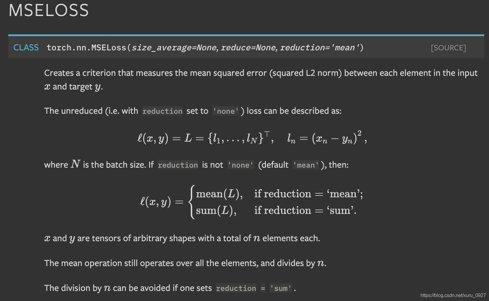
大体流程

用了10个.mat，让train为6个，test为4个，batch_size=2

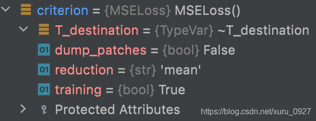
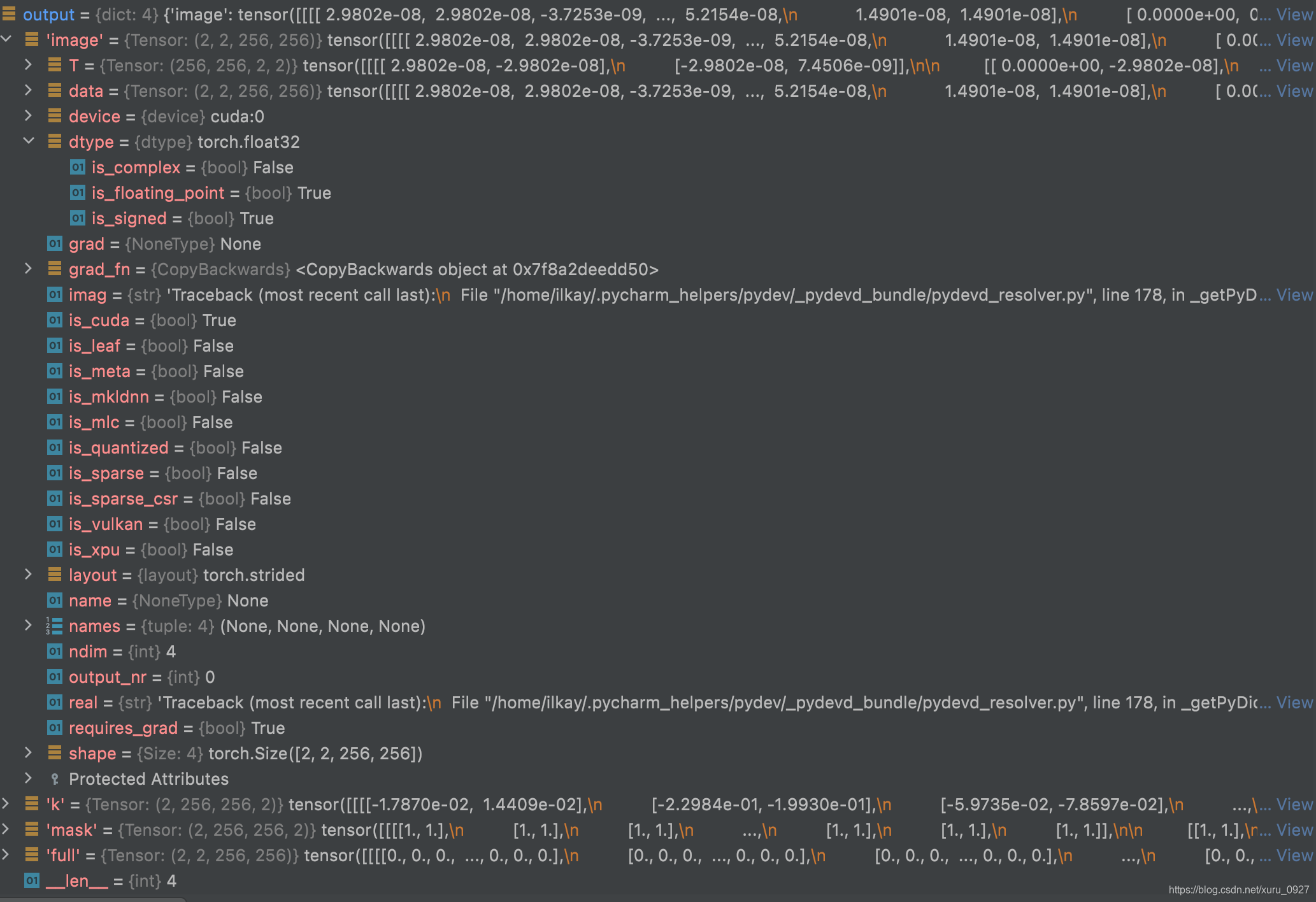
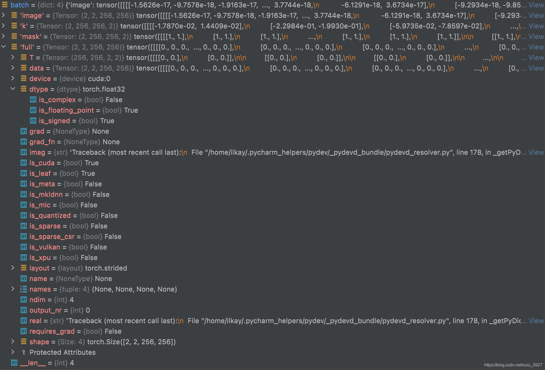
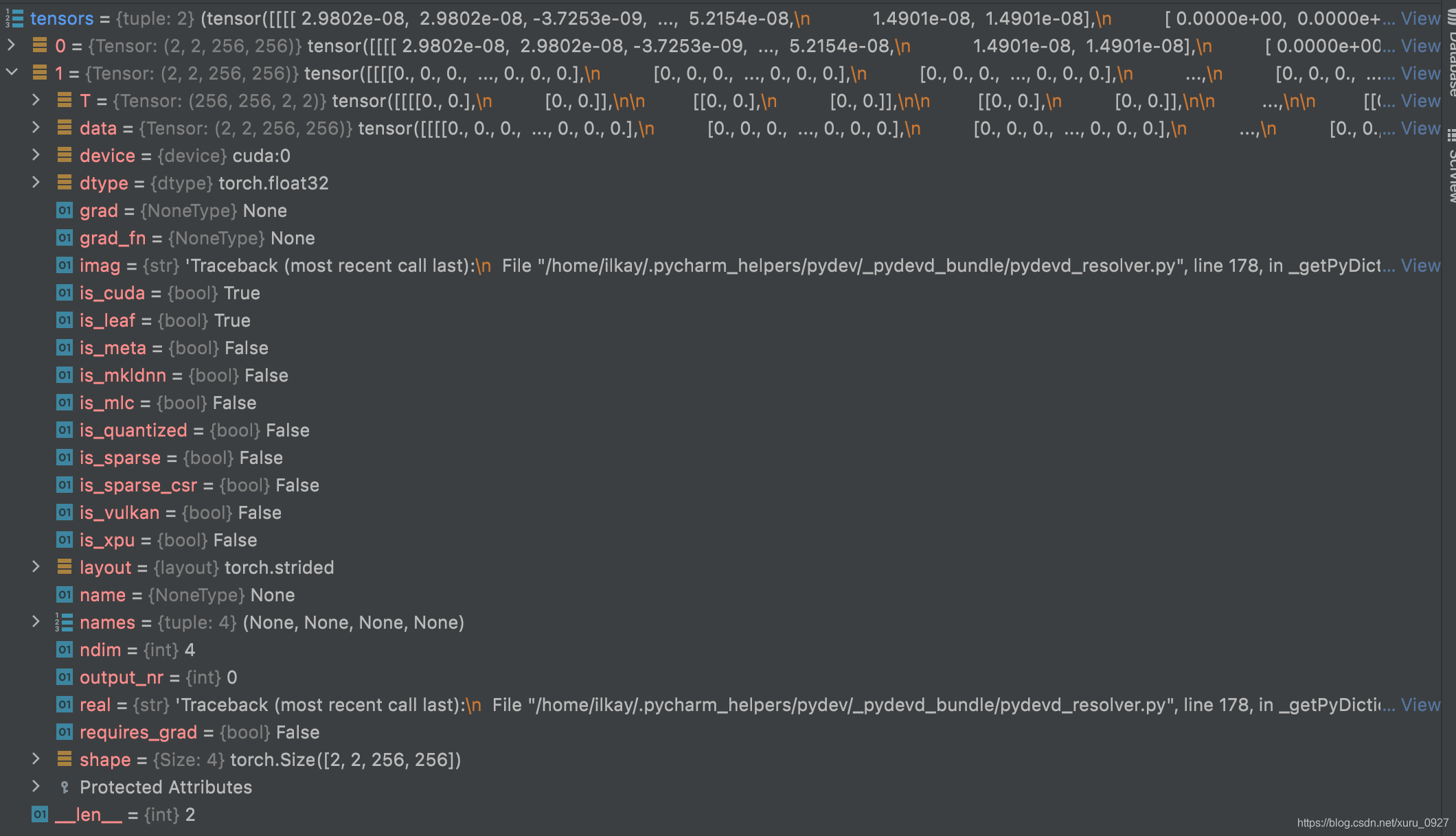
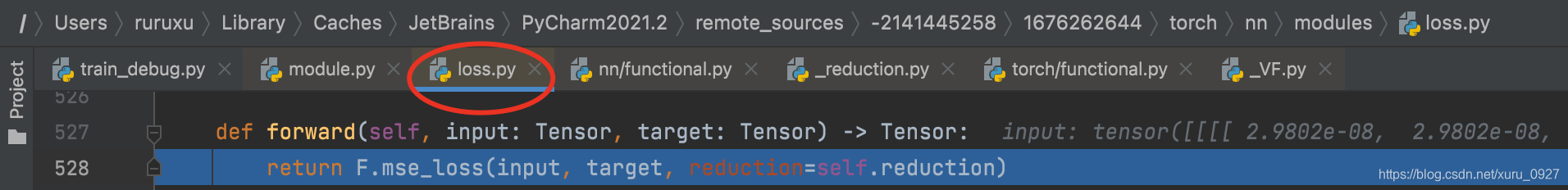
loss = criterion(output['image'], batch['full'])

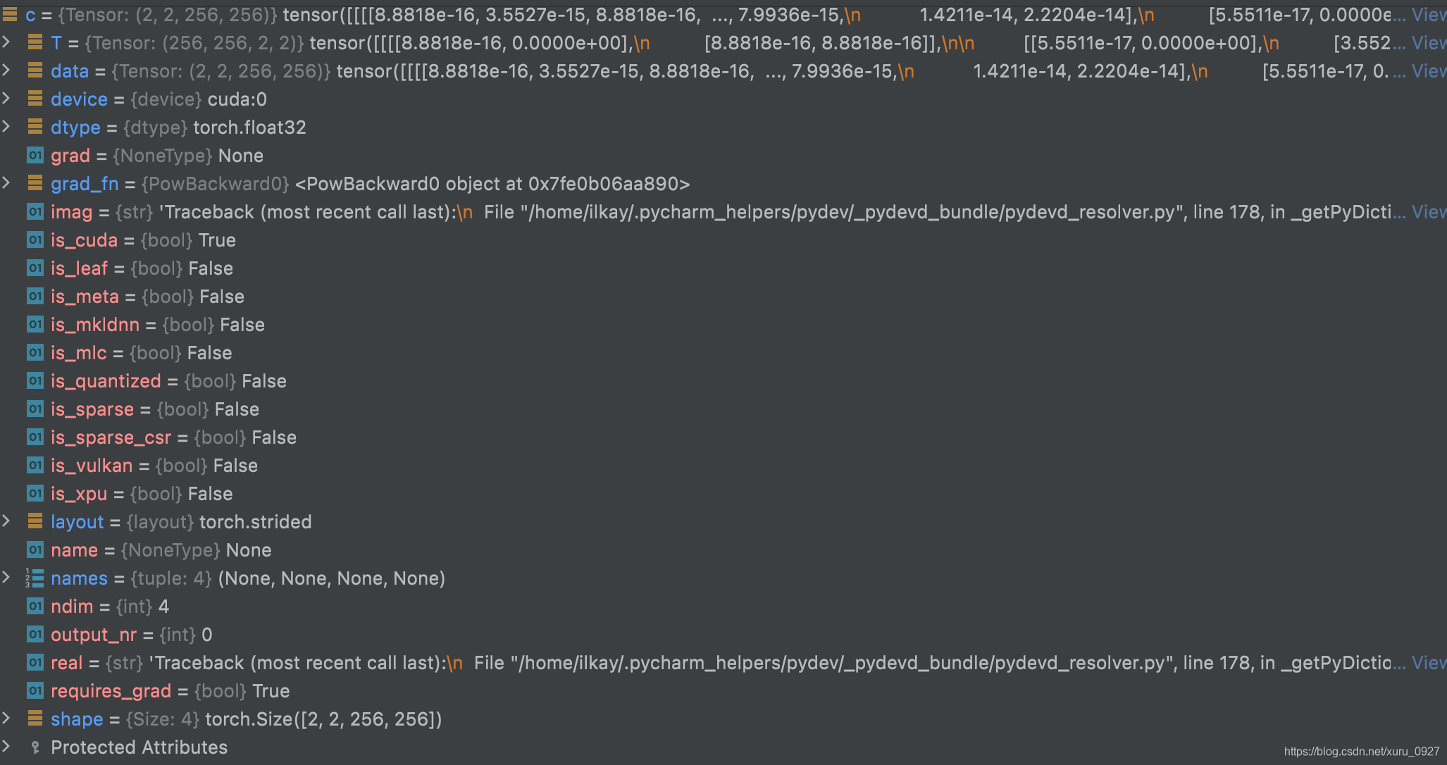
执行loss跳到这里

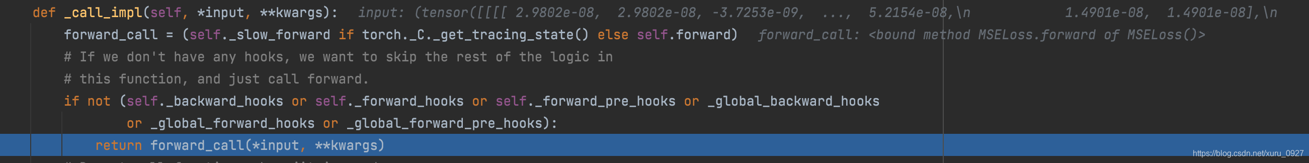
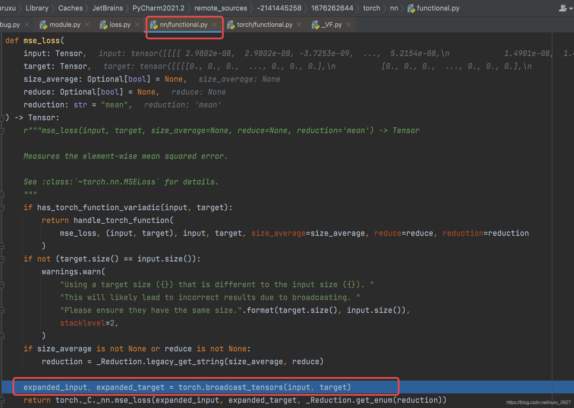
再跳到这里

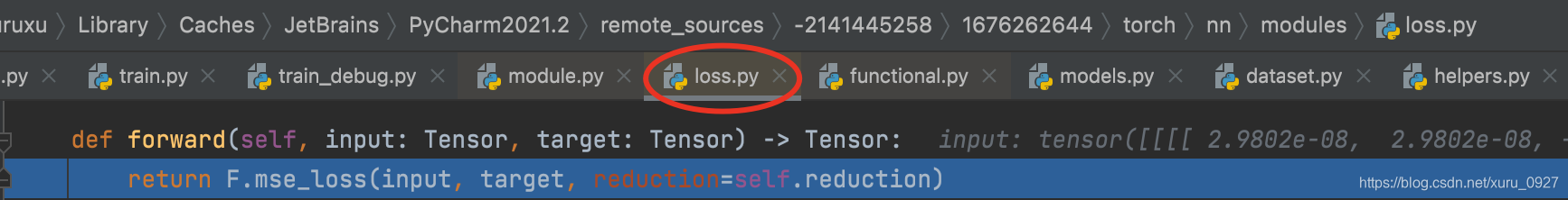
再跳到这里

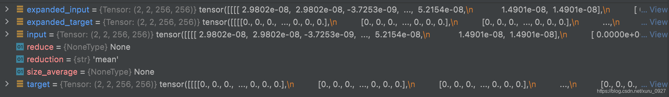
再跳到这里


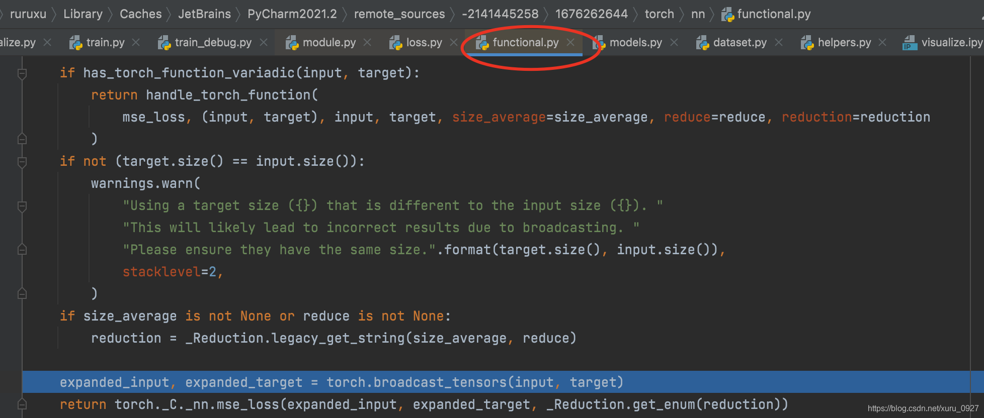
跳到这里


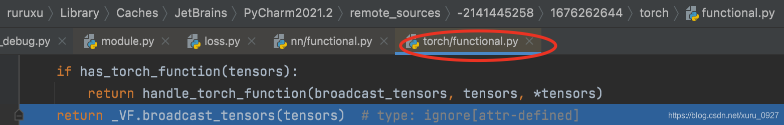
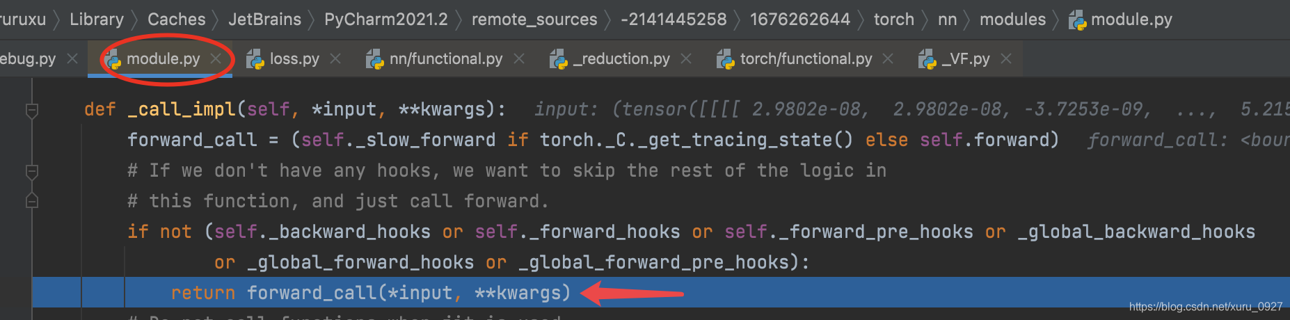
执行上面的return语句时跳到这里

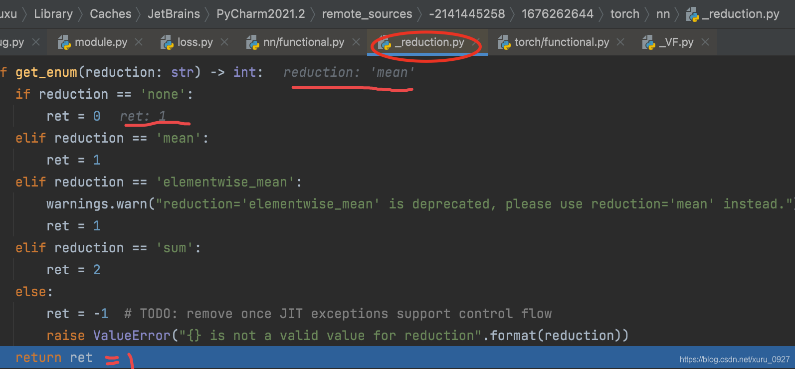
然后return结束返回到原位置


跳回到原来的位置


回到最原始的loss语句

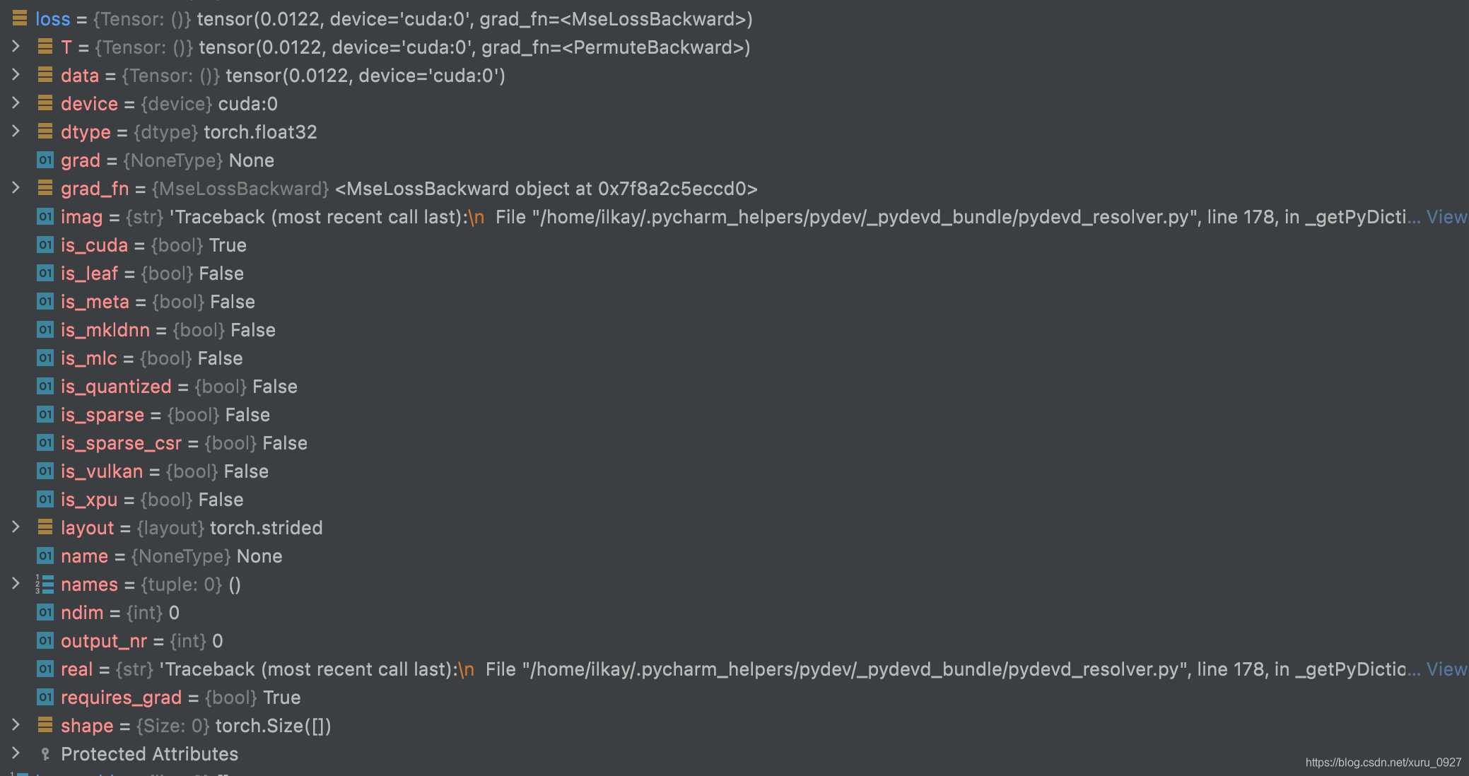
手动计算

粗略手动计算调torch

import torch
a = output['image']
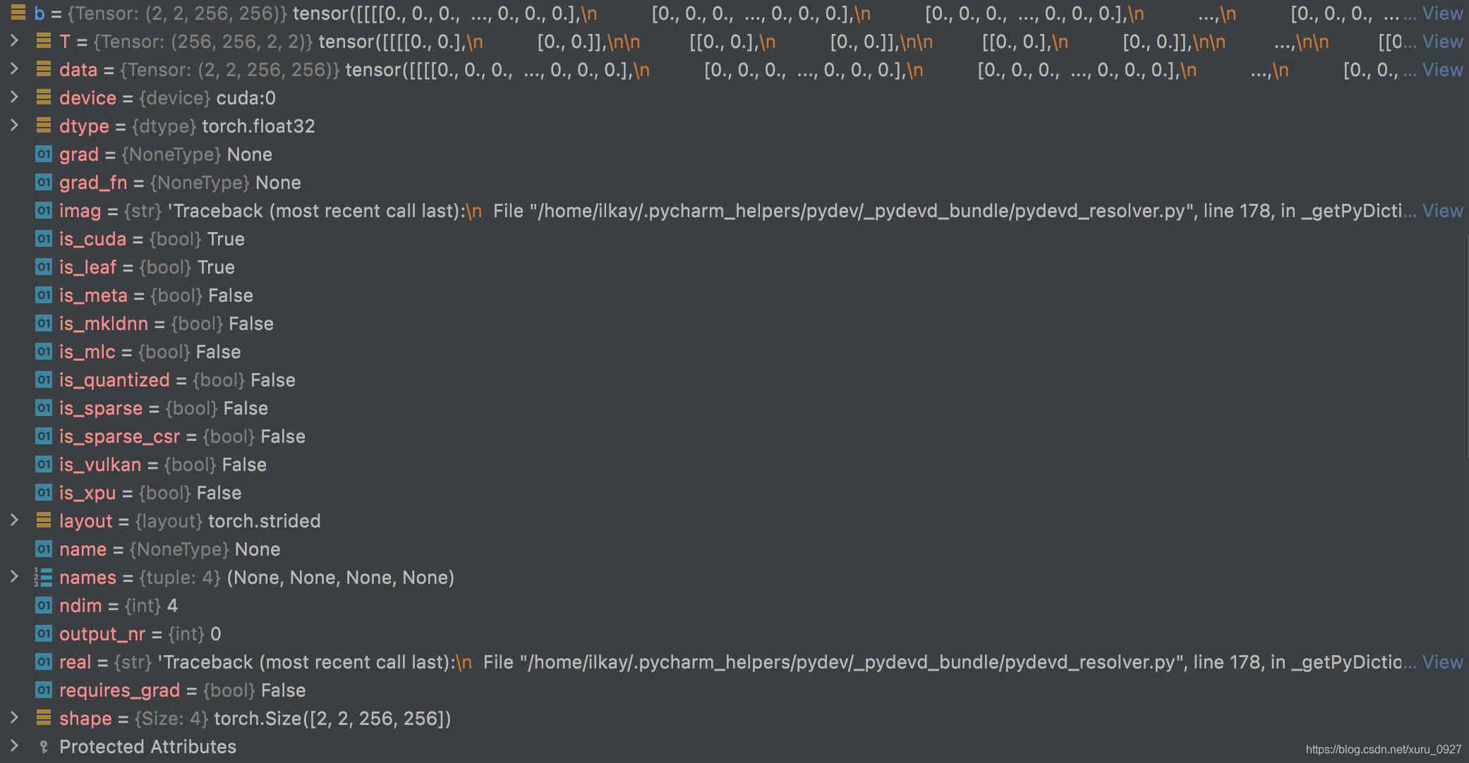
b = batch['full']
c = torch.square(a-b)
torch.mean(c)

output：
tensor(0.0089, device='cuda:0', grad_fn=<MeanBackward0>)

step by step手动计算用numpy

a0_0 = a[0,0, :,:].cpu().detach().numpy()
a0_1 = a[0,1, :,:].cpu().detach().numpy()
a1_0 = a[1,0, :,:].cpu().detach().numpy()
a1_1 = a[1,1, :,:].cpu().detach().numpy()

b0_0 = b[0,0, :,:].cpu().detach().numpy()
b0_1 = b[0,1, :,:].cpu().detach().numpy()
b1_0 = b[1,0, :,:].cpu().detach().numpy()
b1_1 = b[1,1, :,:].cpu().detach().numpy()

c0_0 = c[0,0, :,:].cpu().detach().numpy()
c0_1 = c[0,1, :,:].cpu().detach().numpy()
c1_0 = c[1,0, :,:].cpu().detach().numpy()
c1_1 = c[1,1, :,:].cpu().detach().numpy()

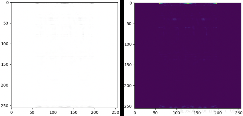
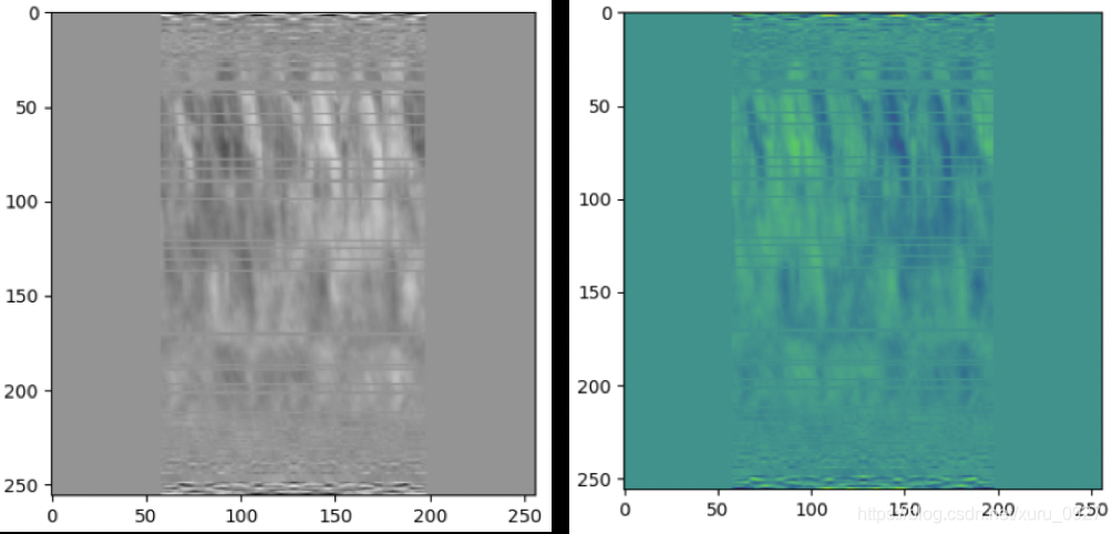
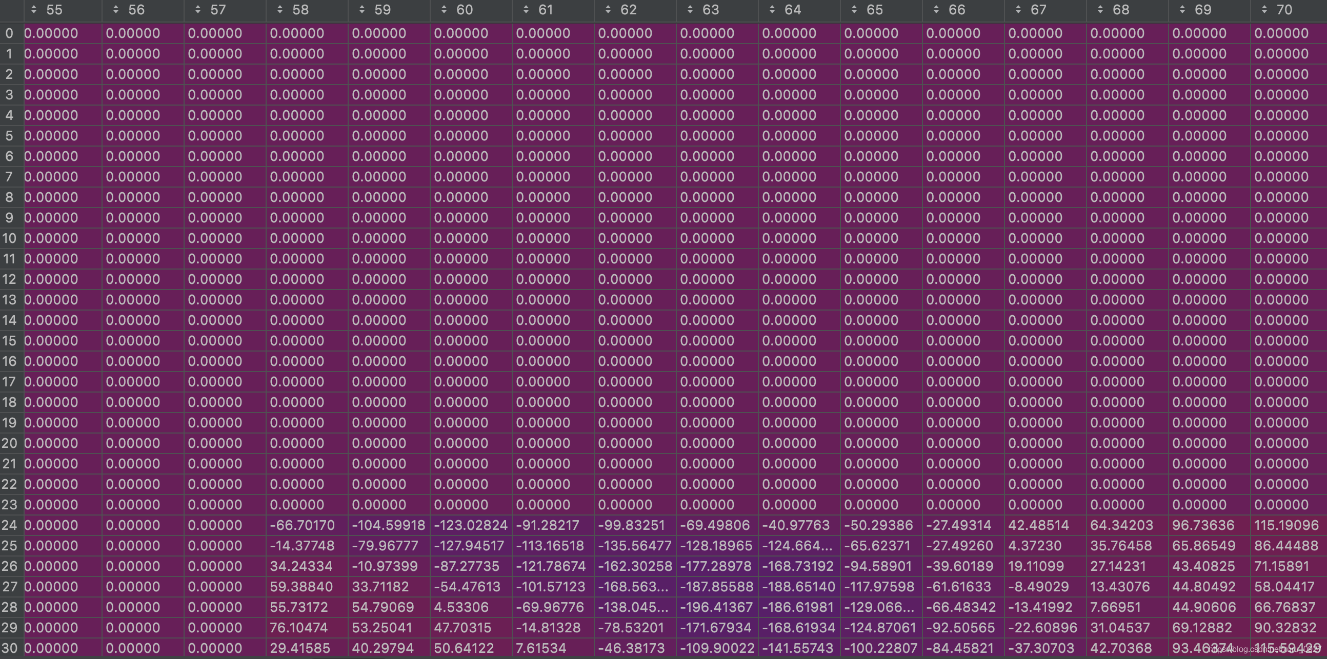
部分a0_0


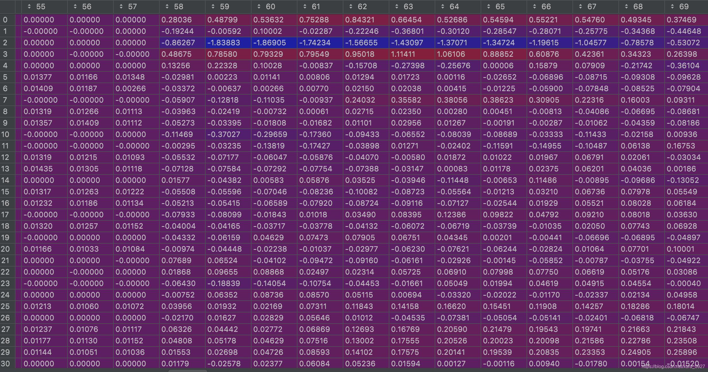
部分b0_0


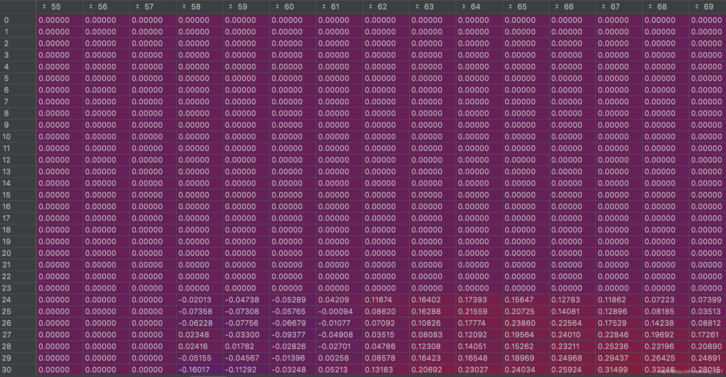
部分c0_0


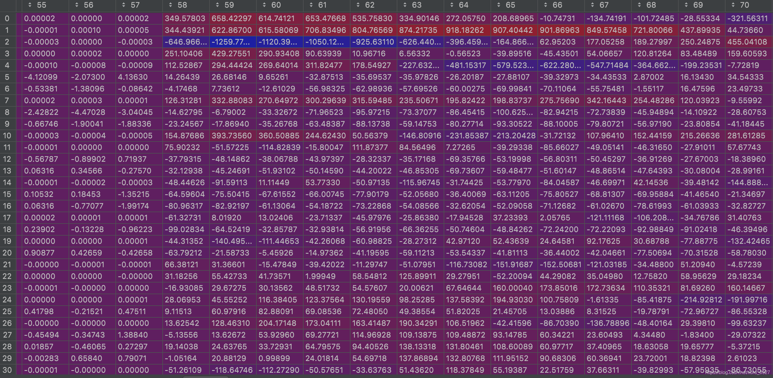
接下来看一下a0_0 - b0_0

ab0_0 = a0_0 - b0_0

部分ab0_0

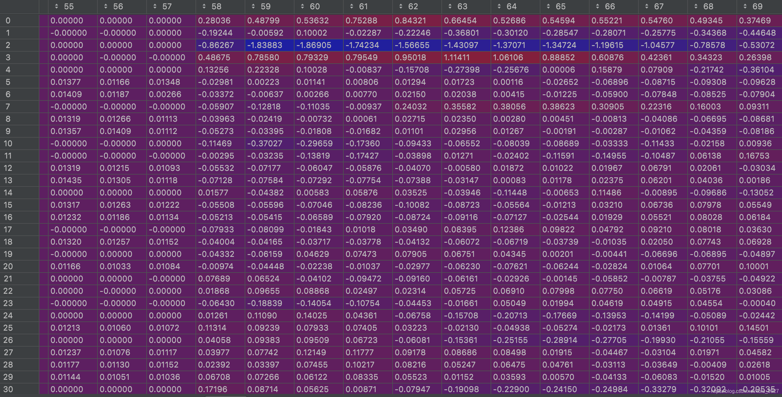
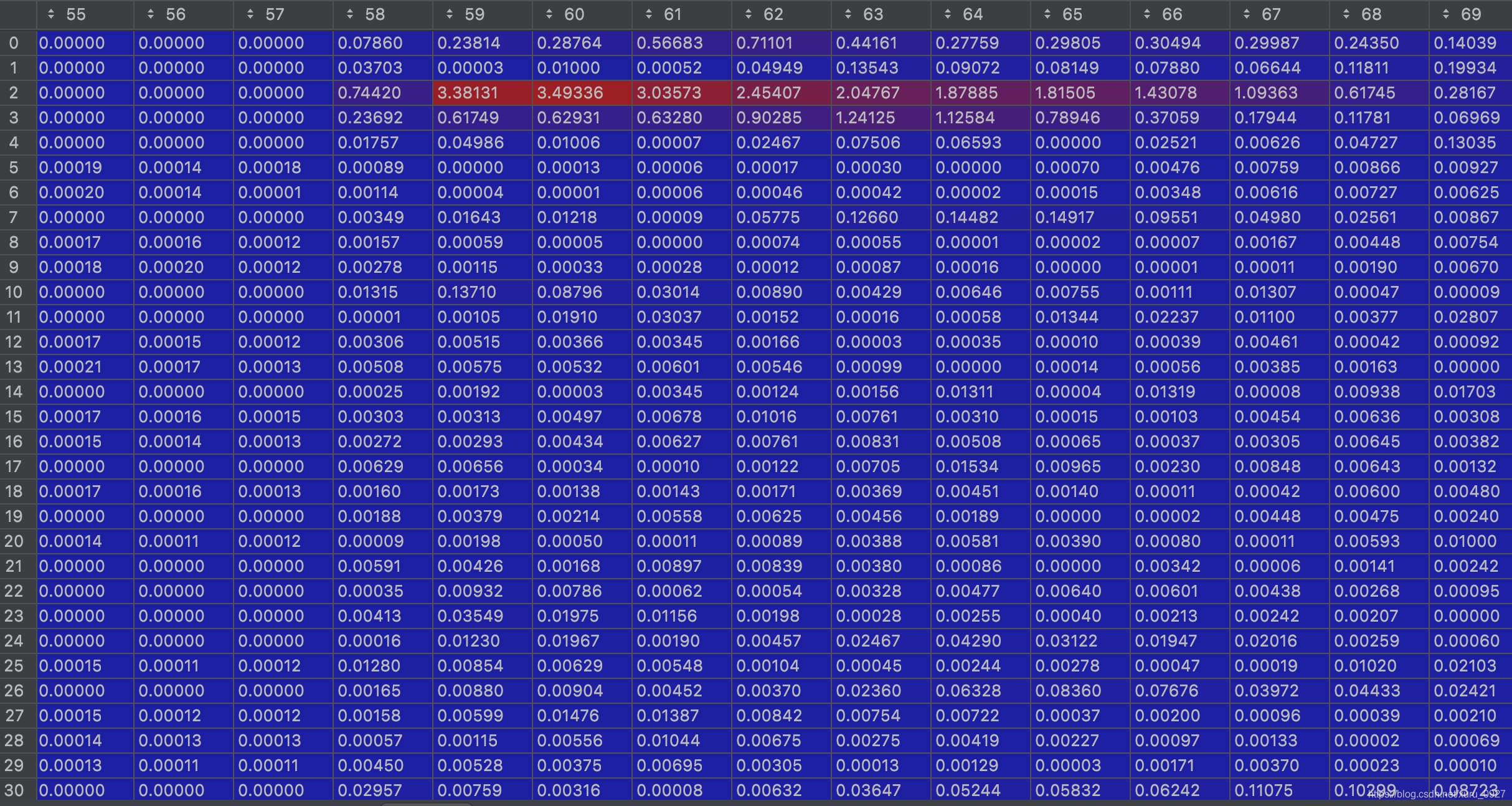
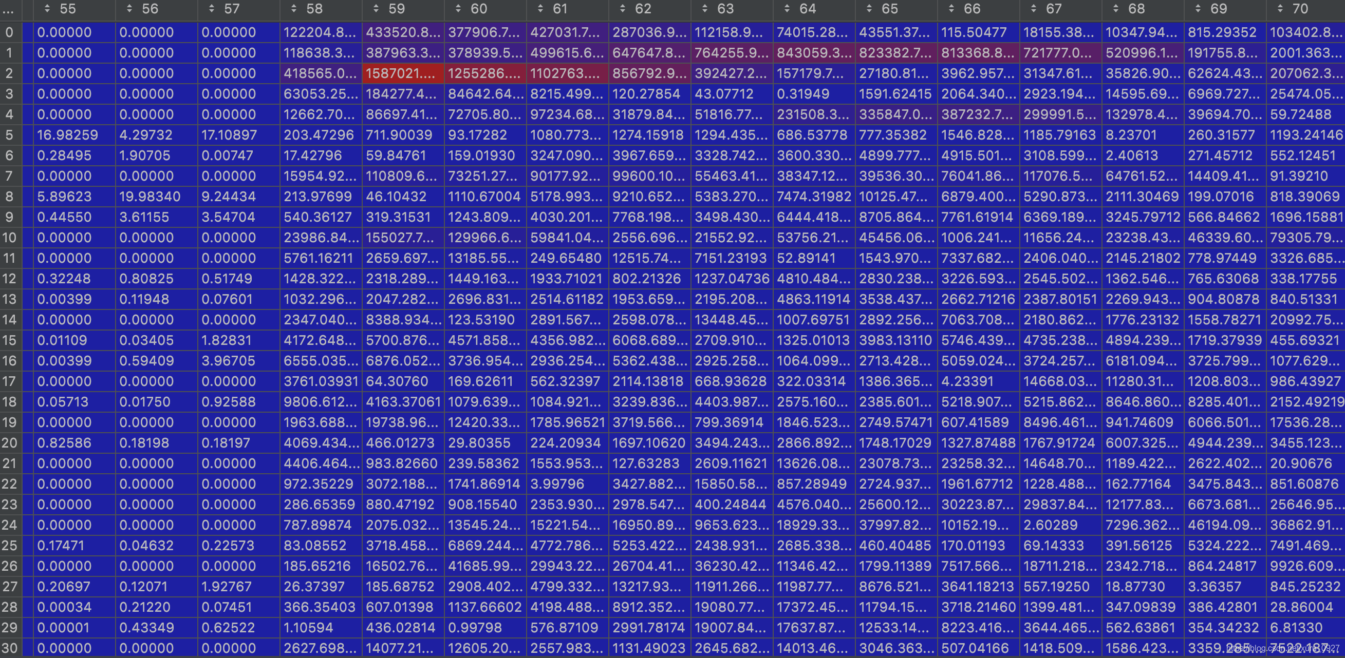
ab0_0_square = np.square(ab0_0)

从图中看出证明成立！！！

np.mean(c0_0) + np.mean(c0_1) + np.mean(c1_0) + np.mean(c1_1)
0.009624282 + 0.011007344 + 0.0072128586 + 0.007779765 = 0.03562425

0.03562425/4 = 0.0089060625证明成立！！！

summary

loss是一个batch一个batch算得。上面的数字是一个batch的结果。

loss+=是把所有batch算出来的数字加和，然后除以batch的个数得到最终的loss。这里10个.mat， train=6个，test=4个，batch_size=2

这里len(dataloaders[phase].dataset)=6
len(dataloaders[phase]）= 3

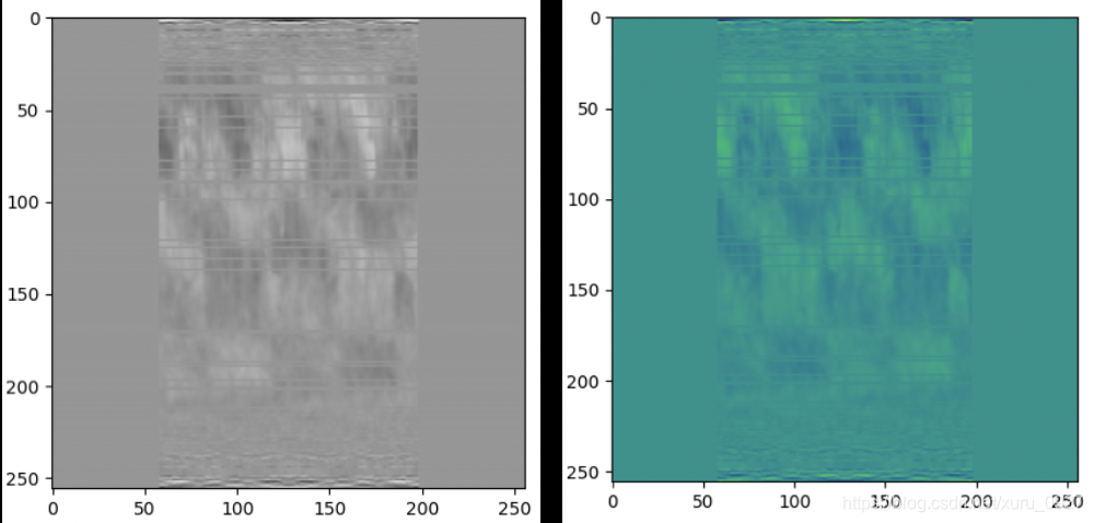
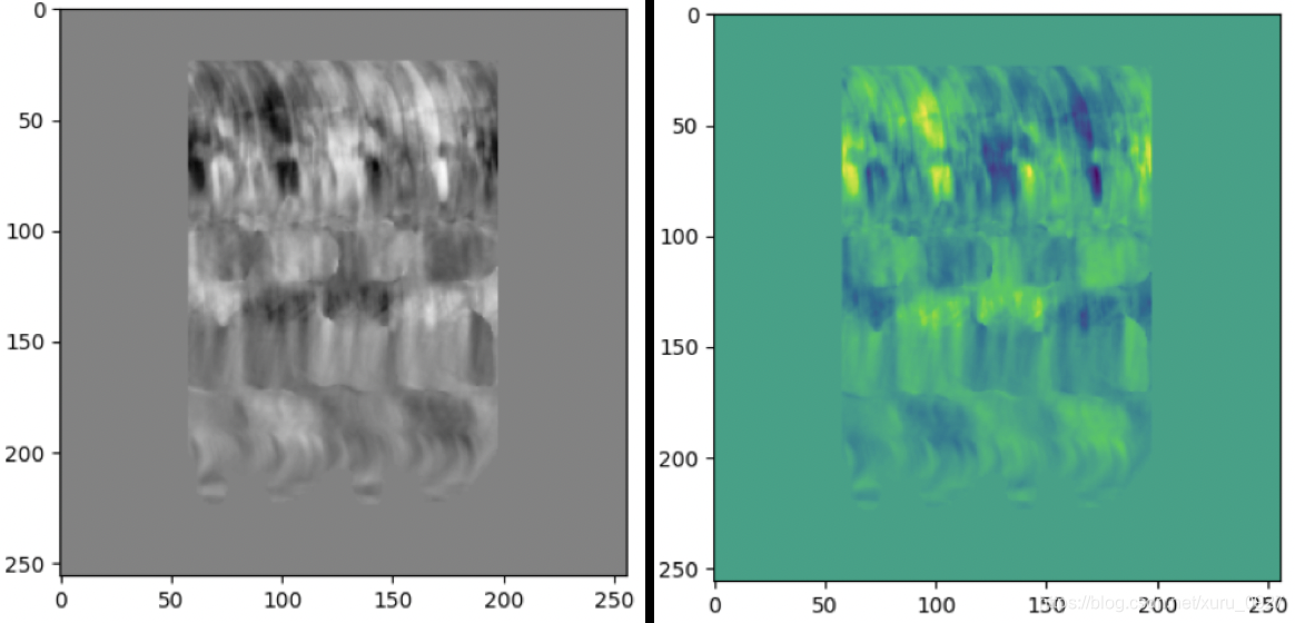
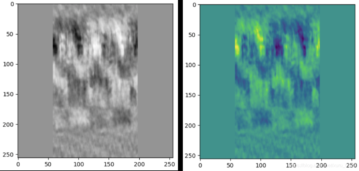
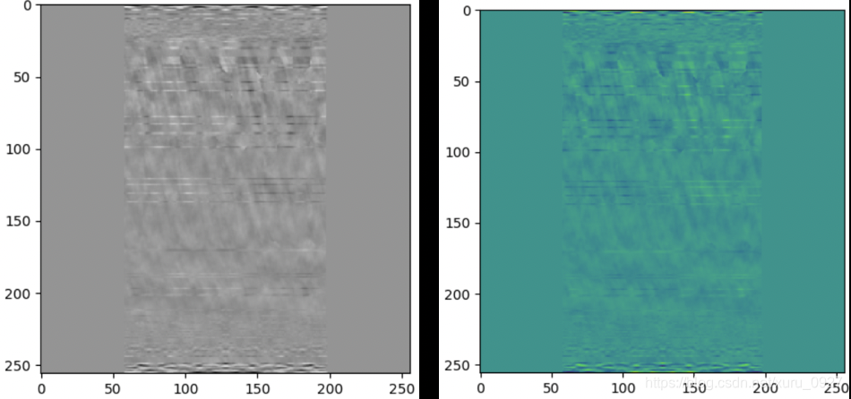
这里也看一下batch[image]

plt.imshow(batch['image'][0,0, :,:].cpu().detach().numpy(),cmap='Greys')

总结

这里我理解了关于loss的三条语句

	loss = criterion(output['image'], batch['full'])
	#bsize=2,即batch_size=2
	running_error += loss.item() * bsize * 1000
#因为上面多乘了2，所以这里除以的不是batch的数量3，而是3*bsize=6，即整个train data的个数
epoch_loss = running_error / len(dataloaders[phase].dataset)

😄😄😄😄😄😄😄😄😄😄😄😄😄😄😄😄😄😄😄😄😄😄😄😄😄😄😄😄
通过上面可以看到数值非常小，不方便观察，下面我把原始数据集的数值扩大1000=1e3倍，再操作一遍
😄😄😄😄😄😄😄😄😄😄😄😄😄😄😄😄😄😄😄😄😄😄😄😄😄😄😄😄

数据集值扩大1000倍

import torch
a = output['image']
b = batch['full']
c = torch.square(a-b)
torch.mean(c)

Out[3]: tensor(8610.2891, device='cuda:0', grad_fn=<MeanBackward0>)

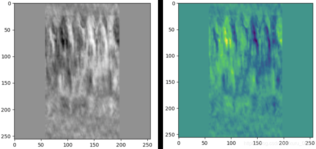
首先看一下batch[image]

plt.imshow(batch['image'][0,0, :,:].cpu().detach().numpy(),cmap='Greys')

a0_0 = a[0,0, :,:].cpu().detach().numpy()
a0_1 = a[0,1, :,:].cpu().detach().numpy()
a1_0 = a[1,0, :,:].cpu().detach().numpy()
a1_1 = a[1,1, :,:].cpu().detach().numpy()

b0_0 = b[0,0, :,:].cpu().detach().numpy()
b0_1 = b[0,1, :,:].cpu().detach().numpy()
b1_0 = b[1,0, :,:].cpu().detach().numpy()
b1_1 = b[1,1, :,:].cpu().detach().numpy()

c0_0 = c[0,0, :,:].cpu().detach().numpy()
c0_1 = c[0,1, :,:].cpu().detach().numpy()
c1_0 = c[1,0, :,:].cpu().detach().numpy()
c1_1 = c[1,1, :,:].cpu().detach().numpy()

部分a0_0


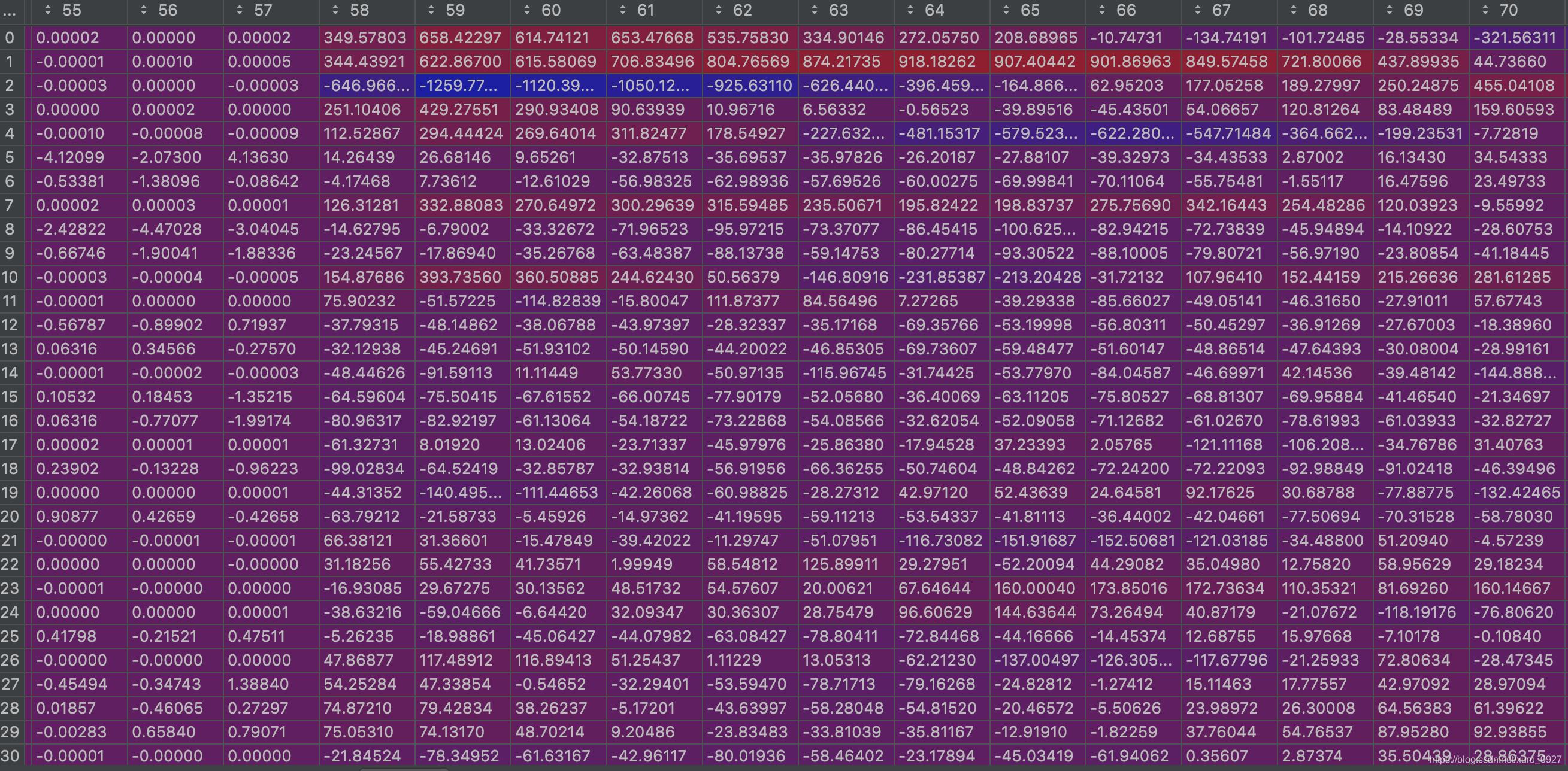
部分b0_0


部分c0_0


接下来看一下a0_0 - b0_0

ab0_0 = a0_0 - b0_0

部分ab0_0

ab0_0_square = np.square(ab0_0)

从图中看出证明成立！！！

np.mean(c0_0) + np.mean(c0_1) + np.mean(c1_0) + np.mean(c1_1)
7608.1436 + 8365.6 + 8671.041 + 9796.372 = 34441.156

34441.156/4 = 8610.289证明成立！！！