tensorflow从入门到放弃---第一篇

案例一

 import tensorflow as tf

 a=3

 w=tf.Variable([[0.5,  1.0 ]])

 x=tf.Variable([ [2, 0], [1, 0] ])

y=tf.matmul(w,x)

print(y)

init_op=tf.global_variables_initializer()

with tf.Session() as sess:

          sess.run(init_op)

          print(y.eval())

最终得出两个结果：

Tersor("Variable_9/read:0",shape(1,2), dtype=float32)

[[2.]]

案例二：

  input1=tf.placeholder(tf.float32)

  input2=tf.placeholder(tf.float32)   #先占上一个地

  output=tf.mul(input1,input2)

  with  tf.Session()  as  sess:

           print(sess.run([ output ],feed_dict={input1:[7.],input2:[2.] } ) )

输出：

[array([14.], dtype=float32)]

案例三：通过tensorflow构造一个线性回归模型

import numpy as np

import tensorflow as tf

import matplotlib.pyplot as plt

 

num_points=1000

vectors_set=[]

for i in range(num_points):

   x1=np.random.normal(0.0,0.55)#对1进行高斯均值初始化，以0为均值，0.55为标准差

   y1=x1*0.1+0.3+np.random.normal(0.0,0.03)

   vectors_set.append([x1,y1])

   

x_data=[v[0] for v in vectors_set]

y_data=[v[1] for v in vectors_set]

 

plt.scatter(x_data,y_data,c='y')

plt.show()

 

#生成1维的W矩阵，取值是[-1,1]之间的随机数

W=tf.Variable(tf.random_uniform([1],-1.0,1.0),name='W')

#生成1维的b矩阵，初始值是0

b=tf.Variable(tf.zeros([1]),name='b')

#经过计算得出预估值y 找到最合适的W和b

y=W*x_data+b  

 

#以估计值y和实际值y_data之间的均方误差作为损失

loss=tf.reduce_mean(tf.square(y-y_data),name='loss')

#采用梯度下降法来优化参数-------优化器

optimizer=tf.train.GradientDescentOptimizer(0.5)

#训练的过程就是最下化这个误差值

train=optimizer.minimize(loss,name='train')

 

sess=tf.Session()

init=tf.global_variables_initializer()

sess.run(init)

#初始化的W和b是多少

print("W=",sess.run(W),"b=",sess.run(b),"loss=",sess.run(loss))

#执行20次训练

for step in range(20):

   sess.run(train)

    #输出训练好的W和b

   print("W=",sess.run(W),"b=",sess.run(b),"loss=",sess.run(loss))

输出：

随着迭代的进行，W越来越接近0.1，b越来越接近0.3，loss值越来越小

案例三：Mnist手写字符识别

import numpy as np
import tensorflow as tf
import matplotlib.pyplot as plt
import input_data

print("packs loaded")

mnist = input_data.read_data_sets('data/',one_hot=True)
trainimg =mnist.train.images
trainlabel=mnist.train.labels
testimg  = mnist.test.images
testlabel= mnist.test.labels
print("MNIST loaded")

print (trainimg.shape)
print (trainlabel.shape)
print (testimg.shape)
print (testlabel.shape)
print (testlabel[0])

x= tf.placeholder("float",[None,784])

y= tf.placeholder("float",[None,10])

W=tf.Variable(tf.zeros([784,10]))
b=tf.Variable(tf.zeros([10]))

actv=tf.nn.softmax(tf.matmul(x,W)+b) #Wx+b  softmax输出结果是概率值
#y*tf.log(actv) 表示真实分类的概率值
cost=tf.reduce_mean(-tf.reduce_sum(y*tf.log(actv),reduction_indices=1))

learning_rate=0.01
optm=tf.train.GradientDescentOptimizer(learning_rate).minimize(cost)

#其中tf.argmax(actv,1) 代表预测值第一行最大数对应的索引值 ，tf.argmax(y,1)真实值对应的索引

#其中tf.argmax(actv,0) 代表预测值第一列最大数对应的索引值 ，tf.argmax(y,0)真实值对应的索引

pred=tf.equal(tf.argmax(actv,1),tf.argmax(y,1))
#pred返回值是True 或者 False
accr=tf.reduce_mean(tf.cast(pred,"float")) #准确率衡量

init= tf.global_variables_initializer()

training_epochs=50  #所有样本进行50次迭代
batch_size=100      #每一次迭代100个样本，每一个batch有100个样本
display_step=5

sess=tf.Session()
sess.run(init)

#MINI-BATCH LEARNING   每一个epoch进行迭代
for epoch in range(training_epochs):
    avg_cost=0.
    num_batch=int(mnist.train.num_examples/batch_size)
    for i in range(num_batch):   #每一个batch进行选择
        #其中batch_xs代表样本，batch_ys代表标签
        batch_xs,batch_ys=mnist.train.next_batch(batch_size)
        sess.run(optm,feed_dict={x:batch_xs,y:batch_ys})
        feeds={x:batch_xs,y:batch_ys}

        #损失函数值
        avg_cost+=sess.run(cost,feed_dict=feeds)/num_batch
    

     #DISPLAY
    if epoch%display_step==0:#每5个epoch打印一下,分别是第5，10，15，20，25，30，35，40，45，50次
        feeds_train={x:batch_xs,y:batch_ys}
        feeds_test ={x:mnist.test.images,y:mnist.test.labels}
        train_acc =sess.run(accr,feed_dict=feeds_train)   #训练的准确率
        test_acc=sess.run(accr,feed_dict=feeds_test)      #测试的准确率
        print("Epch: %03d/%03d cost:%.9f train_acc: %.3f test_acc:%.3f"
        %(epoch,training_epochs,avg_cost,train_acc,test_acc))

print("Done")

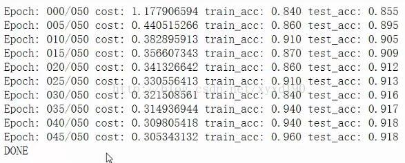
输出结果：

案例四：通过tensorflow实现一个简单的神经网络

import numpy as np
import tensorflow as tf
import matplotlib.pyplot as plt
import input_data

mnist = input_data.read_data_sets('data/', one_hot=True)

# NETWORK TOPOLOGIES
n_hidden_1 = 256    #第一层有256个神经元
n_hidden_2 = 128    #第二层有128个神经元
n_input    = 784       
n_classes  = 10  


# INPUTS AND OUTPUTS
x = tf.placeholder("float", [None, n_input])
y = tf.placeholder("float", [None, n_classes])
    
# NETWORK PARAMETERS
stddev = 0.1
weights = {
    'w1': tf.Variable(tf.random_normal([n_input, n_hidden_1], stddev=stddev)),          #w1是784*256
    'w2': tf.Variable(tf.random_normal([n_hidden_1, n_hidden_2], stddev=stddev)),   #w2是256*128
    'out': tf.Variable(tf.random_normal([n_hidden_2, n_classes], stddev=stddev))      #out是128*10
}
biases = {
    'b1': tf.Variable(tf.random_normal([n_hidden_1])),         #b1是256维
    'b2': tf.Variable(tf.random_normal([n_hidden_2])),         #b2是128维
    'out': tf.Variable(tf.random_normal([n_classes]))            #out是10维
}
print ("NETWORK READY")

def multilayer_perceptron(_X, _weights, _biases):
    layer_1 = tf.nn.sigmoid(tf.add(tf.matmul(_X, _weights['w1']), _biases['b1'])) 
    layer_2 = tf.nn.sigmoid(tf.add(tf.matmul(layer_1, _weights['w2']), _biases['b2']))
    return (tf.matmul(layer_2, _weights['out']) + _biases['out'])

# PREDICTION
pred = multilayer_perceptron(x, weights, biases)

# LOSS AND OPTIMIZER
cost = tf.reduce_mean(tf.nn.softmax_cross_entropy_with_logits(pred, y)) 
optm = tf.train.GradientDescentOptimizer(learning_rate=0.001).minimize(cost)        #通过梯度下降法是的Loss函数最小
corr = tf.equal(tf.argmax(pred, 1), tf.argmax(y, 1))       #corr只用两个值，TRUE和FALSE
accr = tf.reduce_mean(tf.cast(corr, "float"))                 #将准确率转换成float类型


# INITIALIZER
init = tf.global_variables_initializer()
print ("FUNCTIONS READY")

training_epochs = 20   #训练迭代20次

batch_size      = 100    #每一个batch有100个样本

display_step    = 4

# LAUNCH THE GRAPH
sess = tf.Session()
sess.run(init)

# OPTIMIZE
for epoch in range(training_epochs):
    avg_cost = 0.
    total_batch = int(mnist.train.num_examples/batch_size)
    # ITERATION
    for i in range(total_batch):
        batch_xs, batch_ys = mnist.train.next_batch(batch_size)
        feeds = {x: batch_xs, y: batch_ys}
        sess.run(optm, feed_dict=feeds)
        avg_cost += sess.run(cost, feed_dict=feeds)
    avg_cost = avg_cost / total_batch

    # DISPLAY
    if (epoch+1) % display_step == 0:
        print ("Epoch: %03d/%03d cost: %.9f" % (epoch, training_epochs, avg_cost))
        feeds = {x: batch_xs, y: batch_ys}
        train_acc = sess.run(accr, feed_dict=feeds)
        print ("TRAIN ACCURACY: %.3f" % (train_acc))
        feeds = {x: mnist.test.images, y: mnist.test.labels}
        test_acc = sess.run(accr, feed_dict=feeds)
        print ("TEST ACCURACY: %.3f" % (test_acc))
print ("OPTIMIZATION FINISHED")