


股票市场一直以来都是投资者和分析师关注的焦点,而预测股票价格则是金融领域最具挑战性的任务之一。随着深度学习技术的快速发展,尤其是长短期记忆网络(LSTM)在时间序列数据上的出色表现,越来越多的研究者开始尝试用LSTM来预测股票价格。本文将带你一步步实现一个基于LSTM的股票价格预测模型,从数据预处理、特征工程到模型训练与验证,最终通过可视化展示预测结果。
1. 引言:为什么选择LSTM?
LSTM(Long Short-Term Memory)是一种特殊的循环神经网络(RNN),它能够捕捉时间序列数据中的长期依赖关系。相比于传统的RNN,LSTM通过引入“记忆单元”和“门控机制”,有效解决了梯度消失和梯度爆炸的问题,因此在处理时间序列数据时表现出色。
股票价格数据具有明显的时间依赖性,过去的价格走势往往会影响未来的价格变化。因此,LSTM非常适合用于股票价格预测任务。
2. 数据准备与预处理
2.1 导入数据
首先,我们需要导入所需的库并加载股票数据。本文使用的数据集是一个包含日期和收盘价的CSV文件。
import numpy as np
import pandas as pd
import matplotlib.pyplot as plt
import seaborn as sns
from sklearn.preprocessing import MinMaxScaler
import torch
import torch.nn as nn
import time
import math
from sklearn.metrics import mean_squared_error
import plotly.express as px
import plotly.graph_objects as go# 导入数据
filepath = './rlData.csv'
data = pd.read_csv(filepath)# 将数据按照日期进行排序,确保时间序列递增
data = data.sort_values('Date')# 打印前几条数据
print(data.head())
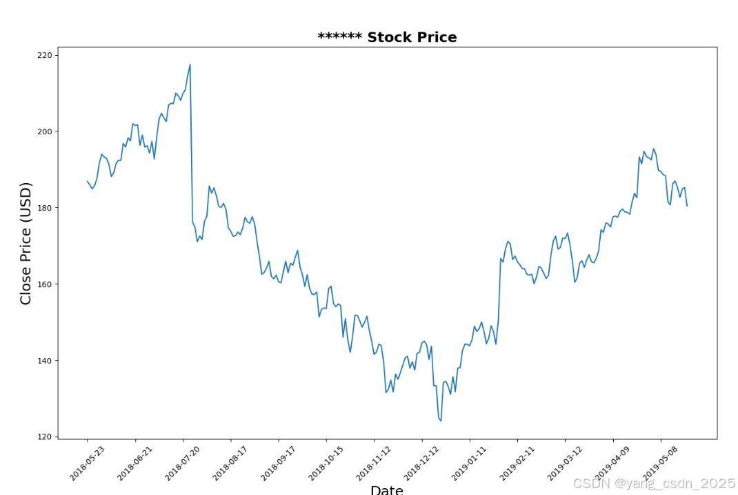
2.2 数据可视化
在开始建模之前,我们首先对股票的收盘价进行可视化,以便更好地理解数据的走势。
plt.figure(figsize=(15, 9))
plt.plot(data['Close'])
plt.xticks(range(0, data.shape[0], 20), data['Date'].loc[::20], rotation=45)
plt.title("****** Stock Price", fontsize=18, fontweight='bold')
plt.xlabel('Date', fontsize=18)
plt.ylabel('Close Price (USD)', fontsize=18)
plt.savefig('StockPrice.jpg')
plt.show()
通过可视化,我们可以直观地看到股票价格的波动情况,这有助于我们判断模型的预测效果。
2.3 特征工程
在时间序列预测中,特征工程是非常重要的一步。我们选择收盘价作为特征,并将其缩放到[-1, 1]之间,以便更好地适应模型的输入。
# 选取Close作为特征
price = data[['Close']]# 进行归一化操作
scaler = MinMaxScaler(feature_range=(-1, 1))
price['Close'] = scaler.fit_transform(price['Close'].values.reshape(-1, 1))
3. 数据集制作
为了训练LSTM模型,我们需要将时间序列数据转换为适合模型输入的格式。具体来说,我们使用过去20天的收盘价来预测第21天的收盘价。
def split_data(stock, lookback):
data_raw = stock.to_numpy()
data = []for index in range(len(data_raw) - lookback):
data.append(data_raw[index: index + lookback])data = np.array(data)
test_set_size = int(np.round(0.2 * data.shape[0]))
train_set_size = data.shape[0] - (test_set_size)x_train = data[:train_set_size, :-1, :]
y_train = data[:train_set_size, -1, :]
x_test = data[train_set_size:, :-1, :]
y_test = data[train_set_size:, -1, :]return [x_train, y_train, x_test, y_test]
lookback = 20
x_train, y_train, x_test, y_test = split_data(price, lookback)
4. 模型构建与训练
4.1 定义LSTM模型
我们使用PyTorch来构建LSTM模型。模型的输入维度为1(收盘价),隐藏层维度为32,输出维度为1(预测的收盘价)。
class LSTM(nn.Module):
def __init__(self, input_dim, hidden_dim, num_layers, output_dim):
super(LSTM, self).__init__()
self.hidden_dim = hidden_dim
self.num_layers = num_layers
self.lstm = nn.LSTM(input_dim, hidden_dim, num_layers, batch_first=True)
self.fc = nn.Linear(hidden_dim, output_dim)def forward(self, x):
h0 = torch.zeros(self.num_layers, x.size(0), self.hidden_dim).requires_grad_()
c0 = torch.zeros(self.num_layers, x.size(0), self.hidden_dim).requires_grad_()
out, (hn, cn) = self.lstm(x, (h0.detach(), c0.detach()))
out = self.fc(out[:, -1, :])
return outmodel = LSTM(input_dim=input_dim, hidden_dim=hidden_dim, output_dim=output_dim, num_layers=num_layers)
4.2 模型训练
我们使用均方误差(MSE)作为损失函数,并使用Adam优化器来训练模型。
criterion = torch.nn.MSELoss()
optimiser = torch.optim.Adam(model.parameters(), lr=0.01)hist = np.zeros(num_epochs)
start_time = time.time()for t in range(num_epochs):
y_train_pred = model(x_train)
loss = criterion(y_train_pred, y_train_lstm)
print("Epoch ", t, "MSE: ", loss.item())
hist[t] = loss.item()
optimiser.zero_grad()
loss.backward()
optimiser.step()training_time = time.time() - start_time
print("Training time: {}".format(training_time))
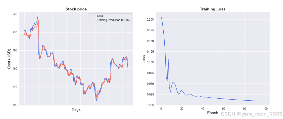
5. 模型结果可视化
训练完成后,我们将预测结果与真实值进行对比,并绘制损失曲线。
sns.set_style("darkgrid")
fig = plt.figure()
fig.subplots_adjust(hspace=0.2, wspace=0.2)plt.subplot(1, 2, 1)
ax = sns.lineplot(x=original.index, y=original[0], label="Data", color='royalblue')
ax = sns.lineplot(x=predict.index, y=predict[0], label="Training Prediction (LSTM)", color='tomato')
ax.set_title('Stock price', size=14, fontweight='bold')
ax.set_xlabel("Days", size=14)
ax.set_ylabel("Cost (USD)", size=14)
ax.set_xticklabels('', size=10)plt.subplot(1, 2, 2)
ax = sns.lineplot(data=hist, color='royalblue')
ax.set_xlabel("Epoch", size=14)
ax.set_ylabel("Loss", size=14)
ax.set_title("Training Loss", size=14, fontweight='bold')fig.set_figheight(6)
fig.set_figwidth(16)
plt.show()
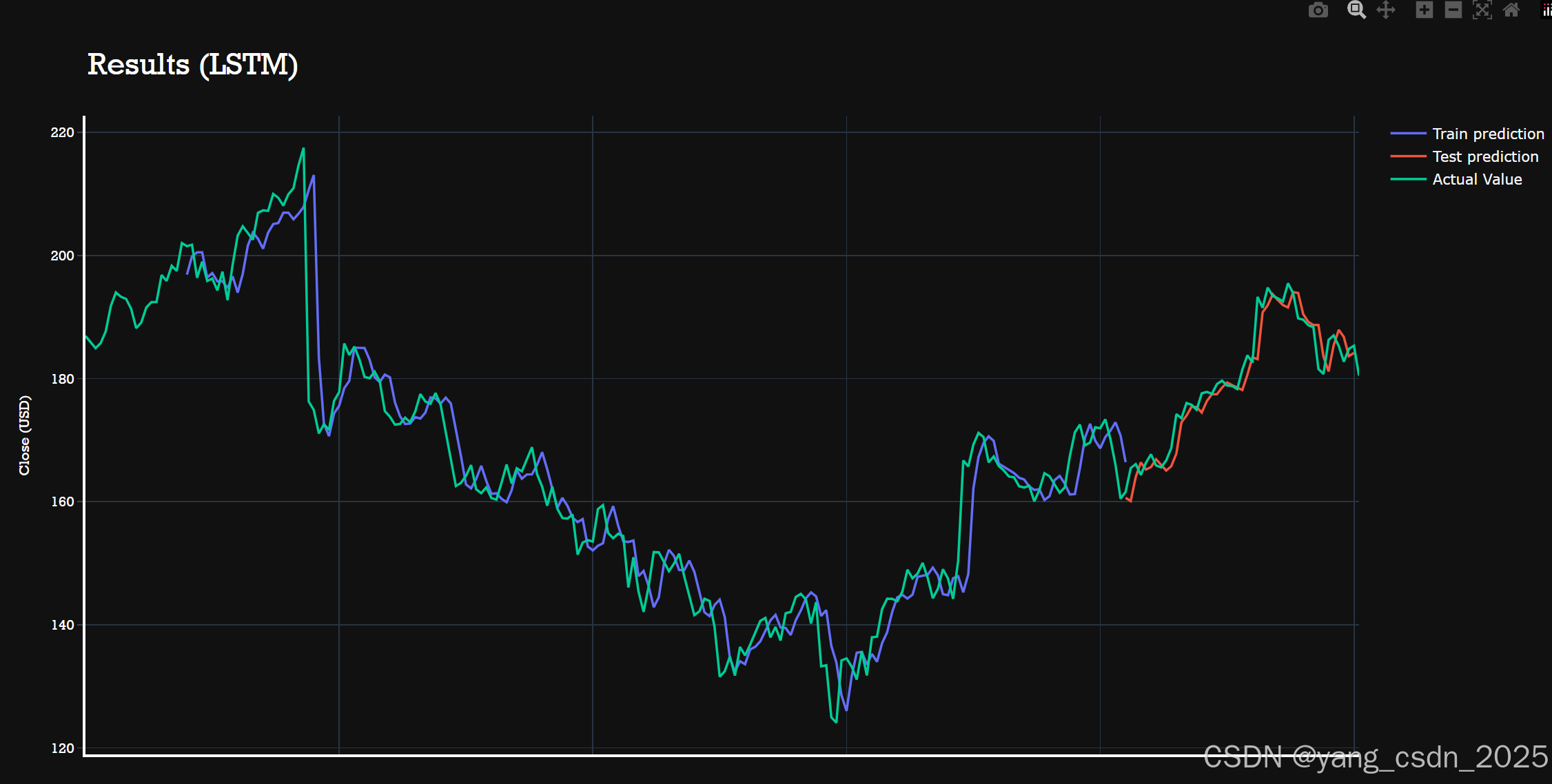
6. 模型验证
最后,我们对模型进行验证,计算训练集和测试集的均方根误差(RMSE),并使用Plotly进行可视化展示。
# 计算均方根误差
trainScore = math.sqrt(mean_squared_error(y_train[:, 0], y_train_pred[:, 0]))
print("Train Score: %.2f RMSE" % (trainScore))
testScore = math.sqrt(mean_squared_error(y_test[:, 0], y_test_pred[:, 0]))
print("Test Score: %.2f RMSE" % (testScore))# 使用Plotly进行可视化
fig = go.Figure()
fig.add_trace(go.Scatter(x=result.index, y=result[0], mode='lines', name='Train prediction'))
fig.add_trace(go.Scatter(x=result.index, y=result[1], mode='lines', name='Test prediction'))
fig.add_trace(go.Scatter(x=result.index, y=result[2], mode='lines', name='Actual Value'))fig.update_layout(
xaxis=dict(
showline=True,
showgrid=True,
showticklabels=False,
linecolor='white',
linewidth=2
),
yaxis=dict(
title_text='Close (USD)',
titlefont=dict(
family='Rockwell',
size=12,
color='white',
),
showline=True,
showgrid=True,
showticklabels=True,
linecolor='white',
linewidth=2,
ticks='outside',
tickfont=dict(
family='Rockwell',
size=12,
color='white',
),
),
showlegend=True,
template='plotly_dark'
)annotations = []
annotations.append(dict(xref='paper', yref='paper', x=0.0, y=1.05,
xanchor='left', yanchor='bottom',
text='Results (LSTM)',
font=dict(family='Rockwell',
size=26,
color='white'),
showarrow=False))fig.update_layout(annotations=annotations)
fig.show()
7. 结论
通过本文的实践,我们成功构建了一个基于LSTM的股票价格预测模型,并对其进行了训练和验证。LSTM在时间序列数据上的表现非常出色,能够有效捕捉股票价格的变化趋势。然而,股票市场受到多种因素的影响,单一模型可能无法完全捕捉所有的市场动态。未来的工作可以尝试结合更多的特征和多模型融合的方法,以进一步提高预测的准确性。
希望本文能够帮助你理解如何使用LSTM进行股票价格预测,并为你的金融数据分析提供一些启发。如果你对代码或模型有任何疑问,欢迎在评论区留言讨论!


 2987
2987

 被折叠的 条评论
为什么被折叠?
被折叠的 条评论
为什么被折叠?
 到【灌水乐园】发言


