


1.导入已知的包:
# Packages import
# Required packages
import numpy as np
import scipy as sp
import pandas as pd
import matplotlib.pyplot as plt
import pyDOE as doe
import sklearn.gaussian_process.kernels as skl
import pymc3 as pm
import theano.tensor as tt
import theano
import time
import seaborn as sns
from tqdm import tqdm
import sys
import psutil
import os
import shutil
import copy
from matplotlib import gridspec
from scipy.stats import multivariate_normal
from mpl_toolkits.mplot3d import Axes3D

import pickle as pkl
import tensorflow as tf
import tensorflow_probability as tfp
2.函数定义
下面的函数是直接从 Variational Calibration 复制而来的
在进行仿真之前运行3、4章的函数:
1. 模拟输入函数
该函数根据给定输入范围和维度内的拉丁超立方体设计或统一设计生成模型/观察的输入。
参数:
- d_input:要生成的输入的维度
- n_input:输入的数量
- lims:Ndarray,每个变量的输入范围,每一行是每个变量的限制
- criterion:“m”,“c”表示超立方体,“uniform”表示均匀设计
返回值:
inpues:n_input * d_input Ndarray 个生成的输入点。
"""产生模拟输入"""
def input_locations(d_input, n_input, lims, criterion = "c"):
    """Simulation inputs generator
    The function generates inputs for model/observations according to latin hypercube design or uniform design within given range and dimension of inputs
    Args:
        d_input: The dimension of inputs to be generated
        n_input: The number of inputs
        lims: Ndarray with the range of inputs for each variable , each row is limits for each var
        criterion: "m", "c" for lating hypercube, "uniform" for uniform design

    Returns:
        inputs: n_input * d_input Ndarray with generated input points.
    """
    if criterion == "uniform":
        inputs = []
        for i in range(d_input):
            inputs = inputs + [np.linspace(lims[i, 0], lims[i, 1], int(n_input ** (1 / d_input)))]
        grid_list = np.meshgrid(*inputs)
        inputs = np.zeros((n_input, d_input))
        for i in range(d_input):
            inputs[:,i] = grid_list[i].flatten()

    else:
        # Data generation
        inputs = doe.lhs(d_input, samples = n_input, criterion = criterion)
        # Transformation for the interval
        for i in range(d_input):
            inputs[:,i] = inputs[:,i] * (lims[i,1] - lims[i, 0]) + lims[i, 0]

    return inputs
2. 生成先验GP的均值和协方差
根据 KOH 校准框架对观测 Y 和模型评估 Z 的数据生成进行训练。
参数:
- input_obs:- 观察输入(Ndarray)
- input_m:- 模型输入的 Ndarray
- d_input:模型输入的维度
- theta:校准参数的真实值
- kernels:包含 3 项的字典:f、delta 和noise kernels
- means:包含 2 个项目的字典:f、delta
返回:
- M:MVN分布的平均向量
- K:MVN分布的协方差矩阵
def gp_mean_cov(input_obs, input_m, d_input, theta, kernels, means):
    """The function generates the mean and convariance function of the prior GP that is
    to be used for triaining data generation of observations Y and model evaluations Z according to
    Kennedy & O'Hagan (2001) framework to calibration.

    Args:
        input_obs: Ndarray with observation inputs.
        input_m: Ndarray with model inputs.
        d_input: The dimension of model inputs.
        theta: True value of calibration parameter
        kernels: A dictionary containing 3 items: f, delta, and noise kernels
        means: A dictionary containing 2 items: f, delta

    Returns:
        M: Mean vector of MVN distribution
        K: Covariance matrix of MVN distribution
    """

    ##### 方差部分
    """核input"""
    theta_stack = np.repeat(theta, len(input_obs))
    theta_stack = theta_stack.reshape((len(input_obs), input_m.shape[1] - d_input), order='F')
    kernel_input = np.concatenate((np.concatenate([input_obs, theta_stack], axis = 1), input_m), axis = 0)

    # 模型 GP 的无噪声基础内核
    kernel_base = kernels["f"]
    K_base = kernel_base(kernel_input)

    # Model discrepancy kernel
    #模型差异核
    if kernels["delta"] != 0:

        zeros = np.zeros((input_m.shape[0], input_obs.shape[1]))
        delta_input = np.concatenate([input_obs, zeros])
        K_delta = kernels["delta"](delta_input)
        # Need to set the non-obs parts of the kernel to be zero
        #需要将内核的非观察部分设置为零
        K_delta[:, input_obs.shape[0]:] = 0
        K_delta[input_obs.shape[0]:, :] = 0
        K_base = K_base + K_delta

    # Add noise to the observations
    #为观察添加噪音
    K = K_base + np.diag([kernels["sigma"] ** 2] * input_obs.shape[0] + [0] * input_m.shape[0])

    ##### Means part  均值部分

    # Obs mean观测均值
    obs_mean = np.array([])
    input_obs_theta = np.concatenate([input_obs, theta_stack], axis = 1)
    for elem in input_obs_theta:
        # First input to mean is x, second input is theta
        obs_mean = np.append(obs_mean, means["f"](elem[:d_input], elem[d_input:]) + means["delta"](elem[:d_input]))

    # Model mean模型均值
    m_mean = np.array([])
    for elem in input_m:
        # First input to mean is x, second input is theta
        m_mean = np.append(m_mean, means["f"](elem[:d_input], elem[d_input:]))

    M = np.concatenate((obs_mean, m_mean))

    return M, K
3. 分布的类族
关于分布的类,用作 1) 变分族,2) 过度分散的族,3) 先验
每个类都包含以下方法:
- __init__(self, param, init)
- sample(self, n_size)
- log_pdf(self, theta)
- log_grad_pdf(self, theta)
3.1 任意维度的平均场高斯族的类
高斯平均场族的参数作为字典传递
参数:
- param: 一个字典,包含两个维度为 (dim,) 的数组条目
- param[“mu”] 是具有独立高斯分布均值的一维 Ndarray
- param[“sigma”] 是一个具有独立高斯分布的 np.log(SDs) 的一维 Ndarray
- dim:族的维度
class gaussian_mean_field_family:
    """Class for a mean field gaussian family of arbitrary dimension"""

    def __init__(self, param, dim):
        """The parameters for the Gaussian mean field family are passed as a dictionary

        Args:
            param: A dictionaray containing two entries with arrays of dimension (dim,)
                 - param["mu"] is a 1-dim Ndarray with the means of independent Gaussian distributions
                 - param["sigma"] is a 1-dim Ndarray with the np.log(SDs) of independent Gaussian distributions
            dim: dimension of the family
        """

        self.mu = param["mu"]
        self.sigma = param["sigma"]
        self.dim = dim

    def sample(self, n_size):
        """Samples from the gaussian mean_field variational family

        Args:
            n_size: the number of samples to be generated
        Returns:
            samle: 2 dimensional NDarray where each row is a single sample from the variational family
        """
        """高斯均值场变分族的样本
         参数:
             n_size:要生成的样本数
         返回值:
             sample:二维 NDarray,其中每一行是来自变分族的单个样本
         """
        sample = np.zeros((n_size, self.dim))
        for i in range(self.dim):
            sample[:, i] = np.random.normal(loc = self.mu[i], scale = self.sigma[i], size = n_size)
        return sample

    def log_pdf(self, theta):
        """Calculates the value of log density of the mean field gaussian family at theta
        计算平均场高斯族在 theta 处的log密度值

        Args:
            theta: 1-dim Ndarray of theta values at which the log density will be evaluated
            theta:将评估对数密度的 theta 值的 1-dim Ndarray
        Returns:
            log_dens: The value of log density at theta
        """

        log_dens = 0
        for i in range(self.dim):
            density = sp.stats.norm(loc = self.mu[i], scale = self.sigma[i])
            log_dens = log_dens + np.log(density.pdf(theta[i]))
        return log_dens

    def grad_log_pdf(self, theta):
        """Calculates the value of score function at theta
        在 theta 处计算得分函数的值

        Args:
            theta: 1-dim Ndarray of theta values at which the log gradient will be evaluated
        Returns:
            gradient: 1-dim Ndarray of len(2 * dim) where gradient[:dim] are the values of score function
                    w.r.t mu and gradient[dim:] are the values of score function w.r.t sigma
        """

        gradient = np.zeros(self.dim * 2)
        for i in range(self.dim):
            # score function w.r.t. mean
            gradient[i] = (theta[i] - self.mu[i]) / (self.sigma[i] ** 2)
            # score function w.r.t. SD
            gradient[i + self.dim] = - 1 / self.sigma[i] + ((theta[i] - self.mu[i]) ** 2) / (self.sigma[i] ** 3)
        return gradient
3.2 具有 np.log(param) 参数化的任意维度的平均场 γ \gamma γ 系列的类
f
(
x
∣
α
,
β
)
=
β
α
Γ
(
α
)
∗
x
α
−
1
∗
exp
(
−
β
∗
x
)
f(x|\alpha, \beta) = \frac{\beta ^ \alpha}{\Gamma(\alpha)} * x ^{\alpha - 1} * \exp({- \beta * x})
f(x∣α,β)=Γ(α)βα∗xα−1∗exp(−β∗x)
E
(
X
)
=
α
/
β
E(X) = \alpha / \beta
E(X)=α/β
V
a
r
(
X
)
=
α
/
(
β
2
)
Var(X) = \alpha / (\beta^2)
Var(X)=α/(β2)
伽马平均场族的参数作为字典传递
参数:
- param: 一个字典,包含两个维度为 (dim,) 的数组条目
- param[“alpha”] 是一个 一维 Ndarray,具有独立 Gamma 分布的 np.log(alpha) 参数
- param[“beta”]是一个 一维 Ndarray,具有独立 Gamma 分布的 np.log(beta) 参数
- dim:族的维度
class gamma_mean_field_family:
    """Class for a mean field gamma family of arbitrary dimension with np.log(param) parametrization

      Gamma parametrization:
      Gamma 参数

          $f(x|alpha, beta) = \frac{beta ^ alpha}{Gamma(alpha)} * x ^{alpha - 1} * \exp{- beta * x}$

          E(X) = alpha / beta
          Var(X) = alpha / (beta^2)

    """

    def __init__(self, param, dim):
        """The parameters for the gamma mean field family are passed as a dictionary

        Args:
            param: A dictionaray containing two entries with arrays of dimension (dim,)
                 - param["alpha"] is a 1-dim Ndarray with the np.log(alpha) parameters of independent Gamma distributions
                 - param["beta"] is a 1-dim Ndarray with the np.log(beta) parameters of independent Gamma distributions
            dim: Dimension of the family
        """

        self.alpha = param["alpha"]
        self.beta = param["beta"]
        self.dim = dim

    def sample(self, n_size):
        """Samples from the gamma mean field variational family

        Note: np.random.gamma has parametrization with shape = alpha, scale = 1 / beta

        Args:
            n_size: the number of samples to be generated
        Returns:
            samle: 2 dimensional NDarray where each row is a single sample from the variational family
        """

        sample = np.zeros((n_size, self.dim))
        for i in range(self.dim):
            sample[:, i] = np.random.gamma(shape = self.alpha[i], scale = self.beta[i], size = n_size)
        return sample

    def log_pdf(self, theta):
        """Calculates the value of log density of the mean field gamma family at theta

        Args:
            theta: 1-dim Ndarray of theta values at which the log density will be evaluated
        Returns:
            log_dens: The value of log density at theta
        """

        log_dens = 0
        for i in range(self.dim):
            log_dens = log_dens + (self.alpha[i] - 1) * np.log(theta[i]) - theta[i] /
            self.beta[i] - self.alpha[i] * np.log(self.beta[i]) - np.log(sp.special.gamma(self.alpha[i]))

        return log_dens

    def grad_log_pdf(self, theta):
        """Calculates the value of score function at theta

        Args:
            theta: 1-dim Ndarray of theta values at which the log gradient will be evaluated
        Returns:
            gradient: 1-dim Ndarray of len(2 * dim) where gradient[:dim] are the values of score function
                    w.r.t alpha and gradient[dim:] are the values of score function w.r.t beta
        """

        gradient = np.zeros(self.dim * 2)
        for i in range(self.dim):
            # score function w.r.t. alpha
            gradient[i] = np.log(theta[i]) - np.log(self.beta[i]) - sp.special.digamma(self.alpha[i])
            # score function w.r.t. beta
            gradient[i + self.dim] = theta[i] / (self.beta[i] ** 2) - self.alpha[i] / self.beta[i]
        return gradient
3.3 具有尺度参数化的任意维度的平均场高斯族的类
λ
=
l
o
g
(
e
x
p
(
σ
)
−
a
)
\lambda = log(exp(\sigma) - a)
λ=log(exp(σ)−a)
参数:
- param: 一个字典,包含两个维度为 (dim,) 的数组条目
- param[“mu”] 是具有独立高斯分布均值的一维 Ndarray
- param[“sigma”] 是一个一维 Ndarray,具有独立高斯分布的变换 sd
- param[“a”] 见参数化
- dim:族的维度
class gaussian_mean_field_family_lambda_param:
    """Class for a mean field gaussian family of arbitrary dimension with scale parametrization

    lambda = log(exp(sigma) - a)

    """
    def __init__(self, param, dim):
        """The parameters for the Gaussian mean field family aare passed as a dictionary

        Args:
            param: A dictionaray containing two entries with arrays of dimension (dim,)
                 - param["mu"] is a 1-dim Ndarray with the means of independent Gaussian distributions
                 - param["sigma"] is a 1-dim Ndarray with the transformed sd of independent Gaussian distributions
                 - param["a"] see parametrization
            dim: Dimension of the family
        """

        self.mu = param["mu"]
        self.sigma = param["sigma"]
        self.a = param["a"]
        self.dim = dim

    def sample(self, n_size):
        """Samples from the gaussian mean_field variational family

        Args:
            n_size: the number of samples to be generated
        Returns:
            samle: 2 dimensional NDarray where each row is a single sample from the variational family
        """

        sample = np.zeros((n_size, self.dim))
        for i in range(self.dim):
            sd = np.log(np.exp(self.sigma[i]) + self.a)
            sample[:, i] = np.random.normal(loc = self.mu[i], scale = sd, size = n_size)
        return sample

    def log_pdf(self, theta):
        """Calculates the value of log density of the mean field gaussian family at theta

        Args:
            theta: 1-dim Ndarray of theta values at which the log density will be evaluated
        Returns:
            log_dens: The value of log density at theta
        """

        log_dens = 0
        for i in range(self.dim):
            sd = np.log(np.exp(self.sigma[i]) + self.a)
            density = sp.stats.norm(loc = self.mu[i], scale = sd)
            log_dens = log_dens + np.log(density.pdf(theta[i]))
        return log_dens

    def grad_log_pdf(self, theta):
        """Calculates the value of score function at theta

        Args:
            theta: 1-dim Ndarray of theta values at which the log gradient will be evaluated
        Returns:
            gradient: 1-dim Ndarray of len(2 * dim) where gradient[:dim] are the values of score function
                    w.r.t mu and gradient[dim:] are the values of score function w.r.t sigma
        """

        gradient = np.zeros(self.dim * 2)
        for i in range(self.dim):
            # score function w.r.t. mean
            gradient[i] = - (self.mu[i] - theta[i]) / (np.log(np.exp(self.sigma[i]) + self.a) ** 2)
            # score function w.r.t. lambda
            gradient[i + self.dim] = np.exp(self.sigma[i]) * (- 1 / (np.log(self.a + np.exp(self.sigma[i])) * (self.a + np.exp(self.sigma[i]))) + \
              ((self.mu[i] - theta[i]) ** 2) /
              ((self.a + np.exp(self.sigma[i])) * np.log(self.a + np.exp(self.sigma[i])) ** 3))
        return gradient
3.4 任意平均场伽马族的类,参数化均值和标准差
此处直接参数化无变换
伽玛参数化:
f ( x ∣ α , β ) = β α Γ ( α ) ∗ x α − 1 ∗ exp ( − β ∗ x ) f(x|\alpha, \beta) = \frac{\beta ^ \alpha}{\Gamma(\alpha)} * x ^{\alpha - 1} * \exp({- \beta * x}) f(x∣α,β)=Γ(α)βα∗xα−1∗exp(−β∗x)
E
(
X
)
=
α
/
β
E(X) = \alpha / \beta
E(X)=α/β
V
a
r
(
X
)
=
α
/
(
β
2
)
Var(X) = \alpha / (\beta^2)
Var(X)=α/(β2)
参数:
- param: 一个字典,包含两个维度为 (dim,) 的数组条目
- param[“alpha”]是具有独立 Gamma 分布的 np.log(alpha) 参数的 1-dim Ndarray
- param[“beta”] 是具有独立 Gamma 分布的 np.log(beta) 参数的 1-dim Ndarray
- param[“a”] 见参数化
- dim:族的维度
class gamma_mean_field_family_ms:
    """Class for a mean field gamma family of arbitrary, parametrized with mean and standard deviation

    Directly parametrized no transformation here

      Gamma parametrization:

          f(x|alpha, beta) = \frac{beta ^ alpha}{Gamma(alpha)} * x ^{alpha - 1} * \exp{- beta * x}

          E(X) = alpha / beta
          Var(X) = alpha / (beta^2)

    """

    def __init__(self, param, dim):
        """The parameters for the gamma mean field family are passed as a dictionary

        Args:
            param: A dictionaray containing two entries with arrays of dimension (dim,)
                 - param["alpha"] is a 1-dim Ndarray with the np.log(alpha) parameters of independent Gamma distributions
                 - param["beta"] is a 1-dim Ndarray with the np.log(beta) parameters of independent Gamma distributions
                 - param["a"] see parametrization
            dim: Dimension of the family
        """

        self.alpha = param["alpha"]
        self.beta = param["beta"]
        self.a = param["a"]
        self.dim = dim

    def sample(self, n_size):
        """Samples from the gamma mean field variational family

        Note: np.random.gamma has parametrization with shape = alpha, scale = 1 / beta

        Args:
            n_size: the number of samples to be generated
        Returns:
            samle: 2 dimensional NDarray where each row is a single sample from the variational family
        """


        sample = np.zeros((n_size, self.dim))
        for i in range(self.dim):
            mu = self.alpha[i]
            sigma = self.beta[i]
            alpha = float(mu/sigma) ** 2
            beta = float(mu/ (sigma**2))
            tfd = tfp.distributions
            tfdGamma = tfd.Gamma(concentration=alpha, rate=beta)
            samples = tfdGamma.sample(n_size)
            sample[:, i] = samples.numpy()
        return sample

    def log_pdf(self, theta):
        """Calculates the value of log density of the mean field gamma family at theta

        Args:
            theta: 1-dim Ndarray of theta values at which the log density will be evaluated
        Returns:
            log_dens: The value of log density at theta
        """

        log_dens = 0
        for i in range(self.dim):

            mu = self.alpha[i]
            sigma = self.beta[i]
            alpha = float(mu/sigma) ** 2
            beta = float(mu/ (sigma**2))
            tfd = tfp.distributions
            tfdGamma = tfd.Gamma(concentration=alpha, rate=beta)
            log_dens = log_dens + float(tfdGamma.log_prob(theta[i]))
        return log_dens

    def grad_log_pdf(self, theta):
        """Calculates the value of score function at theta

        Args:
            theta: 1-dim Ndarray of theta values at which the log density will be evaluated
        Returns:
            gradient: 1-dim Ndarray of len(2 * dim) where gradient[:dim] are the values of score function
                    w.r.t alpha and gradient[dim:] are the values of score function w.r.t beta
        """

        gradient = np.zeros(self.dim * 2)
        for i in range(self.dim):
            # score function w.r.t. np.log(alpha)
            l_m = self.alpha[i]
            l_s = self.beta[i]

            gradient[i] = (l_m - theta[i] + 2 * l_m * np.log(theta[i]) + 2 * l_m * np.log(l_m / (l_s ** 2)) - 2 * l_m * sp.special.digamma((l_m/l_s) ** 2)) / (l_s ** 2)

            gradient[i + self.dim] = 2 * (l_m * theta[i] - l_m ** 2 + sp.special.digamma((l_m/l_s)** 2) * l_m ** 2 - np.log(theta[i]) * l_m ** 2 - np.log(l_m / (l_s ** 2)) * l_m **2) / (l_s ** 3)
        return gradient
3.5 任意平均场伽马族的类,参数化均值和标准差
f ( x ∣ α , β ) = β α Γ ( α ) ∗ x α − 1 ∗ exp ( − b e t a ∗ x ) s f(x|\alpha, \beta) = \frac{\beta ^ \alpha}{\Gamma(\alpha)} * x ^{\alpha - 1} * \exp({- beta * x})s f(x∣α,β)=Γ(α)βα∗xα−1∗exp(−beta∗x)s
E
(
X
)
=
α
/
β
E(X) = \alpha / \beta
E(X)=α/β
V
a
r
(
X
)
=
α
/
(
β
2
)
Var(X) = \alpha / (\beta^2)
Var(X)=α/(β2)
参数:
- param: 一个字典,包含两个维度为 (dim,) 的数组条目
- param[“alpha”]是具有独立 Gamma 分布的 np.log(alpha) 参数的 1-dim Ndarray
- param[“beta”] 是具有独立 Gamma 分布的 np.log(beta) 参数的 1-dim Ndarray
- param[“a”] 见参数化
- dim:族的维度
- tau: 色散系数 >= 1
class gamma_mean_field_family_ms_overdisp:
    """Class for a mean field gamma family of arbitrary, parametrized with mean and standard deviation
    directly

      Gamma parametrization:

          f(x|alpha, beta) = \frac{beta ^ alpha}{Gamma(alpha)} * x ^{alpha - 1} * \exp{- beta * x}

          E(X) = alpha / beta
          Var(X) = alpha / (beta^2)

    """

    def __init__(self, param, dim, tau):
        """The parameters for the gamma mean field family are passed as a dictionary

        Args:
            param: A dictionaray containing two entries with arrays of dimension (dim,)
                 - param["alpha"] is a 1-dim Ndarray with the np.log(alpha) parameters of independent Gamma distributions
                 - param["beta"] is a 1-dim Ndarray with the np.log(beta) parameters of independent Gamma distributions
                 - param["a"] see parametrization
            dim: Dimension of the family
            tau: Dispersion coefficient >= 1
        """

        self.alpha = param["alpha"]
        self.beta = param["beta"]
        self.a = param["a"]
        self.tau = tau
        self.dim = dim

    def sample(self, n_size):
        """Samples from the gamma mean field variational family

        Note: np.random.gamma has parametrization with shape = alpha, scale = 1 / beta

        Args:
            n_size: the number of samples to be generated
        Returns:
            samle: 2 dimensional NDarray where each row is a single sample from the variational family
        """


        sample = np.zeros((n_size, self.dim))
        for i in range(self.dim):
            mu = self.alpha[i]
            sigma = self.beta[i]
            alpha = (float(mu/sigma) ** 2 + self.tau[i] - 1) / self.tau[i]
            beta = float(mu/ (sigma**2)) / self.tau[i]
            tfd = tfp.distributions
            tfdGamma = tfd.Gamma(concentration=alpha, rate=beta)
            samples = tfdGamma.sample(n_size)
            sample[:, i] = samples.numpy()
        return sample

    def log_pdf(self, theta):
        """Calculates the value of log density of the mean field gamma family at theta

        Args:
            theta: 1-dim Ndarray of theta values at which the log density will be evaluated
        Returns:
            log_dens: The value of log density at theta
        """

        log_dens = 0
        for i in range(self.dim):

            mu = self.alpha[i]
            sigma = self.beta[i]
            alpha = (float(mu/sigma) ** 2 + self.tau[i] - 1) / self.tau[i]
            beta = float(mu/ (sigma**2)) / self.tau[i]
            tfd = tfp.distributions
            tfdGamma = tfd.Gamma(concentration=alpha, rate=beta)
            log_dens = log_dens + float(tfdGamma.log_prob(theta[i]))
        return log_dens

    def grad_log_pdf_tau(self, theta):
        """Calculate the value of score function at theta w.r.t dispersion coefficient tau

        Args:
            theta: 1-dim Ndarray of theta values at which the log gradient will be evaluated
        Returns:
            gradient: 1-dim Ndarray of len(dim) with the values of score function
                    w.r.t tau
        """
        gradient = np.zeros(self.dim)
        for i in range(self.dim):
            mu = self.alpha[i]
            sigma = self.beta[i]
            alpha = float(mu/sigma) ** 2
            beta = float(mu/ (sigma**2))

            gradient[i] = (self.tau[i] * np.log(beta / self.tau[i]) - (alpha + self.tau[i] - 1) + beta * theta[i] - \
                          np.log(beta / self.tau[i]) * (alpha + self.tau[i] - 1) + sp.special.digamma((alpha + self.tau[i] - 1) /self.tau[i]) * (alpha - 1) - \
                          np.log(theta[i]) * (alpha - 1)) / self.tau[i]
        return gradient
3.6 具有尺度参数化的任意维度的平均场过分散高斯族的类
class gaussian_mean_field_family_lambda_param_overdisp:
    """Class for a mean field overdispersed gaussian family of arbitrary dimension with scale parametrization

    lambda = log(exp(sigma) - a)

    """
    def __init__(self, param, dim, tau):
        """The parameters for the Gaussian mean field family aare passed as a dictionary

        Args:
            param: A dictionaray containing two entries with arrays of dimension (dim,)
                 - param["mu"] is a 1-dim Ndarray with the means of independent Gaussian distributions
                 - param["sigma"] is a 1-dim Ndarray with the np.log(SDs) of independent Gaussian distributions
                 - param["a"] see parametrization
            dim: Dimension of the family
            tau: Dispersion coefficient >= 1
        """

        self.mu = param["mu"]
        self.sigma = param["sigma"]
        self.a = param["a"]
        self.tau = tau
        self.dim = dim

    def sample(self, n_size):
        """Samples from the gaussian mean_field variational family

        Args:
            n_size: the number of samples to be generated
        Returns:
            samle: 2 dimensional NDarray where each row is a single sample from the variational family
        """

        sample = np.zeros((n_size, self.dim))
        for i in range(self.dim):
            sd = np.log(np.exp(self.sigma[i]) + self.a) * np.sqrt(self.tau[i])
            sample[:, i] = np.random.normal(loc = self.mu[i], scale = sd , size = n_size)
        return sample

    def log_pdf(self, theta):
        """Calculates the value of log density of the mean field gaussian family at theta

        Args:
            theta: 1-dim Ndarray of theta values at which the log density will be evaluated
        Returns:
            log_dens: The value of log density at theta
        """

        log_dens = 0
        for i in range(self.dim):
            sd = np.log(np.exp(self.sigma[i]) + self.a) * np.sqrt(self.tau[i])
            density = sp.stats.norm(loc = self.mu[i], scale = sd)
            log_dens = log_dens + np.log(density.pdf(theta[i]))
        return log_dens

    def grad_log_pdf_tau(self, theta):
        """"Calculate the value of score function at theta w.r.t dispersion coefficient tau

        Args:
            theta: 1-dim Ndarray of theta values at which the log gradient will be evaluated
        Returns:
            gradient: 1-dim Ndarray of len(dim) with the values of score function
                    w.r.t tau
        """
        gradient = np.zeros(self.dim)
        for i in range(self.dim):
            sd = np.log(np.exp(self.sigma[i]) + self.a)
            gradient[i] = - 1/(2 * self.tau[i]) + (((theta[i] - self.mu[i]) / (self.tau[i] * sd)) ** 2) / 2

        return gradient
3.7平均场过度分散的任意伽马族的类,参数化均值和标准差
class gamma_mean_field_family_lambda_param_overdisp:
    """Class for a mean field overdispersed gamma family of arbitrary, parametrized with mean and standard deviation

        lambda_alfa = log(exp(alfa) - a)
        lambda_beta = log(exp(alfa) - a)

        where alpha corresponds to the mean of the gamma distribution and beta corresponds to the std of the gamma dist

      Gamma parametrization:

          f(x|alpha, beta) = \frac{beta ^ alpha}{Gamma(alpha)} * x ^{alpha - 1} * \exp{- beta * x}

          E(X) = alpha / beta
          Var(X) = alpha / (beta^2)

    """

    def __init__(self, param, dim, tau):
        """The parameters for the gamma mean field family are passed as a dictionary

        Args:
            param: A dictionaray containing two entries with arrays of dimension (dim,)
                 - param["alpha"] is a 1-dim Ndarray with the np.log(alpha) parameters of independent Gamma distributions
                 - param["beta"] is a 1-dim Ndarray with the np.log(beta) parameters of independent Gamma distributions
                 - param["a"] see above
            tau: Overdispersion parameter value
        """

        self.alpha = param["alpha"]
        self.beta = param["beta"]
        self.a = param["a"]
        self.tau = tau
        self.dim = dim

    def sample(self, n_size):
        """Samples from the gamma mean field variational family

        Note: np.random.gamma has parametrization with shape = alpha, scale = 1 / beta

        Args:
            n_size: the number of samples to be generated
        Returns:
            samle: 2 dimensional NDarray where each row is a single sample from the variational family
        """


        sample = np.zeros((n_size, self.dim))
        for i in range(self.dim):
            mu = np.log(np.exp(self.alpha[i]) + self.a)
            sigma = np.log(np.exp(self.beta[i]) + self.a)
            alpha = (float(mu/sigma) ** 2 + self.tau[i] - 1) / self.tau[i]
            beta = float(mu/ (sigma**2)) / self.tau[i]
            tfd = tfp.distributions
            tfdGamma = tfd.Gamma(concentration=alpha, rate=beta)
            samples = tfdGamma.sample(n_size)
            sample[:, i] = samples.numpy()
        return sample

    def log_pdf(self, theta):
        """Calculates the value of log density of the mean field gamma family at theta

        Args:
            theta: 1-dim Ndarray of theta values at which the log density will be evaluated
        Returns:
            log_dens: The value of log density at theta
        """

        log_dens = 0
        for i in range(self.dim):

            mu = np.log(np.exp(self.alpha[i]) + self.a)
            sigma = np.log(np.exp(self.beta[i]) + self.a)
            alpha = (float(mu/sigma) ** 2 + self.tau[i] - 1) / self.tau[i]
            beta = float(mu/ (sigma**2)) / self.tau[i]
            tfd = tfp.distributions
            tfdGamma = tfd.Gamma(concentration=alpha, rate=beta)
            log_dens = log_dens + float(tfdGamma.log_prob(theta[i]))
        return log_dens


    def grad_log_pdf_tau(self, theta):
        """"Calculate the value of score function at theta w.r.t dispersion coefficient tau

        Args:
            theta: 1-dim Ndarray of theta values at which the log gradient will be evaluated
        Returns:
            gradient: 1-dim Ndarray of len(dim) with the values of score function
                    w.r.t tau
        """

        gradient = np.zeros(self.dim)
        for i in range(self.dim):
            mu = np.log(np.exp(self.alpha[i]) + self.a)
            sigma = np.log(np.exp(self.beta[i]) + self.a)
            alpha = (float(mu/sigma) ** 2)
            beta = float(mu/ (sigma**2))

            gradient[i] = (self.tau[i] * np.log(beta / self.tau[i]) - (alpha + self.tau[i] - 1) + beta * theta[i] - \
                          np.log(beta / self.tau[i]) * (alpha + self.tau[i] - 1) + sp.special.digamma((alpha + self.tau[i] - 1) /self.tau[i]) * (alpha - 1) - \
                          np.log(theta[i]) * (alpha - 1)) / self.tau[i]
        return gradient
4.GP模型均值类定义
4.1模型差异 GP 的均值函数
表示模型差异 GP 的均值函数的通用类
参数
- 超参数:均值的超参数字典
方法
- Zero mean: m ( x ) = 0 m(x) = 0 m(x)=0
- Constant mean: m ( x ) = β m(x) = \beta m(x)=β
- Linear mean: m ( x ) = I n t e r c e p t + β ∗ x T m(x) =Intercept + \beta * x^T m(x)=Intercept+β∗xT
class delta_mean:
    def __init__(self, hyperparametrs):
        """General class representing the mean function of model discrepancy GP

        Args:
            hyperparameters: A dictionary of hyperparameters for the mean
        """
        self.hyperparameters = hyperparametrs

    def zero(self, x):
        """Zero mean: m(x) = 0

        Args:
            x: 1-dim Ndarray of model imputs (or scalar)
        Returns: 0
        """
        return 0

    def constant(self, x):
        """Constant mean: m(x) = \Beta

        Args:
            x: 1-dim Ndarray of model imputs (or scalar)
            self.hyperparameters: A scalar with dictionary key "Beta"
        Returns: self.hyperparameters["Beta"]
        """
        return self.hyperparameters["Beta"]

    def linear(self, x):
        """Linear mean: m(x) =Intercept + \Beta * x^T

        Args:
            x: 1-dim Ndarray of model imputs (or scalar)
            self.hyperparameters: A scalar with dictionary key "Intercept" and a vector of parameters
                                  with dictionary key "Beta" of the same length as lengt(x)
        Returns:
            mean: Intercept + \Beta * (x, theta)^T
        """
        mean = self.hyperparameters["Intercept"] + np.dot(self.hyperparameters["Beta"], x)
        return mean
4.2 计算机模型 GP 的均值函数
表示计算机模型 GP 的均值函数的通用类
参数
- 超参数:均值的超参数字典
方法
- Zero mean: m ( x ) = 0 m(x) = 0 m(x)=0
- Constant mean: m ( x ) = β m(x) = \beta m(x)=β
- dot_product: m ( x , θ ) = β ∗ ( θ 1 ∗ c o s ( x 1 ) + θ 2 ∗ c o s ( x 2 ) ) m(x,\theta) = \beta * (\theta_1 * cos(x_1) + \theta_2 * cos(x_2)) m(x,θ)=β∗(θ1∗cos(x1)+θ2∗cos(x2))
```python
class model_mean:
    def __init__(self, hyperparametrs):
        """General class representing the mean function of computer model GP

        Args:
            hyperparameters: A dictionary of hyperparameters for the mean
        """
        self.hyperparameters = hyperparametrs

    def zero(self, x, theta):
        """Zero mean: m(x,theta) = 0

        Args:
            x: 1-dim Ndarray of model imputs (or scalar)
            theta: 1-dim Ndarray (or scalar) of calibration parameters
        Returns: 0
        """
        return 0

    def constant(self, x, theta):
        """Constant mean: m(x,theta) = \Beta

        Args:
            x: 1-dim Ndarray of model imputs (or scalar)
            theta: 1-dim Ndarray (or scalar) of calibration parameters
            self.hyperparameters: A scalar with dictionary key "Beta"
        Returns: self.hyperparameters["Beta"]
        """
        return self.hyperparameters["Beta"]

    def dot_product(self, x, theta):
        """Dot product mean, for two dimensional model input x as defined in the
           simulation setup in Kejzlar and Maiti (2020):

           m(x,theta) = \Beta * (\theta_1 * cos(x_1) + \theta_2 * cos(x_2))

        Args:
            x: 1-dim Ndarray of model imputs (or scalar)
            theta: 1-dim Ndarray (or scalar) of calibration parameter
            self.hyperparameters: A scalar with dictionary key "Beta"
        Returns: self.hyperparameters["Beta"] * np.dot(x, theta)
        """
        if x.ndim == 1:
            return self.hyperparameters["Beta"] * np.dot(np.array([np.cos(x[0]), np.sin(x[1])]), theta)
        else:
            return self.hyperparameters["Beta"] * np.dot(np.array([np.cos(x[:,0]), np.sin(x[:,1])]), theta)
3.MCMC 贝叶斯校准 - 模拟
此块包含对模拟研究执行 MCMC 校准的代码,
变分方法的代码在 Variational_calibration.ipynb notebook 中
1. 生成训练数据并定义先验分布
准备
priors_dictionary = {}
theta_dim = 2
ns = 30 #Numerators for eta_f and eta_delta
tf.random.set_seed(123)
np.random.seed(123)
- 定义先验分布
- 设置 θ \theta θ 先验
### Theta prior
mean_theta = np.array([0.5,0.5])
cov_theta = np.array([1/10,1/10])
dim = theta_dim
theta_prior = gaussian_mean_field_family(param = {"mu": mean_theta, "sigma": cov_theta}, dim = dim)
"""作为先验分布样本的真实 theta 值"""
theta = theta_prior.sample(1).flatten() # The true theta value as a sample from prior distribution
priors_dictionary["theta"] = theta_prior
- 设置噪声先验
### Noise prior
alpha = np.array([1])
beta = np.array([1/80])
dim = 1
noise_prior = gamma_mean_field_family(param = {"alpha": alpha, "beta": beta}, dim = dim)
noise = np.array([0.01]) # Noise value for simulation
priors_dictionary["sigma"] = noise_prior
- f f f 的核超参数先验
-------- 长度刻度 f l f_l fl 先验
## length scales
alpha = np.array([1])
beta = np.array([20])
beta = np.array([1/4])
dim = 1
kernel_f_l_prior = gamma_mean_field_family(param = {"alpha": alpha, "beta": beta}, dim = dim)
kernel_f_l = 1 # true value of length scale
priors_dictionary["kernel_f_l"] = kernel_f_l_prior
-------- f η f_\eta fη 先验
## eta
alpha = np.array([1])
beta = np.array([1/40])
dim = 1
kernel_f_eta_prior = gamma_mean_field_family(param = {"alpha": alpha, "beta": beta}, dim = dim)
kernel_f_eta = 1/ns # true value of eta_f
priors_dictionary["kernel_f_eta"] = kernel_f_eta_prior
- δ \delta δ 的核超参数先验
-------- 长度刻度 δ l \delta_l δl 先验
## length scales
alpha = np.array([1])
beta = np.array([1/4])
dim = 1
kernel_delta_l_prior = gamma_mean_field_family(param = {"alpha": alpha, "beta": beta}, dim = dim)
kernel_delta_l = 1/2 # true vaule of lenght scale
priors_dictionary["kernel_delta_l"] = kernel_delta_l_prior
-------- δ η \delta_\eta δη 先验
alpha = np.array([1])
beta = np.array([1/40])
dim = 1
kernel_delta_eta_prior = gamma_mean_field_family(param = {"alpha": alpha, "beta": beta}, dim = dim)
kernel_delta_eta = 1/ns # true value of delta_eta
priors_dictionary["kernel_delta_eta"] = kernel_delta_eta_prior
- f f f的均值超参数
f_beta = 1
- δ \delta δ 的均值超参数
### Mean delta hyperparameters
mean_beta = np.array([0])
cov_beta = np.array([1/4])
dim = 1
mean_delta_prior = gaussian_mean_field_family(param = {"mu": mean_beta, "sigma": cov_beta}, dim = dim)
delta_beta = 0.15 # true value of beta
priors_dictionary["mean_delta"] = mean_delta_prior
- 核定义
-------- f f f 核
# f kernel
kernel = {"sq_quad": [kernel_f_eta, kernel_f_l]}
kernel_type = list(kernel)[0]
if kernel_type == "sq_quad":
    kernel_f = float(kernel[kernel_type][0]) ** 2 * skl.RBF(length_scale = kernel[kernel_type][1])

if kernel_type == "matern": # option for mattern kernel
    kernel_f = float(kernel[kernel_type][0]) ** 2 * skl.Matern(length_scale = kernel[kernel_type][1],
                                                               nu = kernel[kernel_type][2])
-------- δ \delta δ 核
# delta kernel
kernel = {"sq_quad": [kernel_delta_eta, kernel_delta_l]} # sigma, l_scale
kernel_type = list(kernel)[0]
if kernel_type == "sq_quad":
    kernel_delta = float(kernel[kernel_type][0]) ** 2 * skl.RBF(length_scale = kernel[kernel_type][1])

if kernel_type == "matern":
    kernel_delta = float(kernel[kernel_type][0]) ** 2 * skl.Matern(length_scale = kernel[kernel_type][1],
                                                               nu = kernel[kernel_type][2])
if kernel_type == "zero":
    kernel_delta = 0
--------- 各种核的输入
kernels_input = {"f":kernel_f, "delta": kernel_delta, "sigma": float(noise)}
kernels = {"f": "sq_quad", "delta": "sq_quad"}
- 均值定义
model_hyperparameters = {"Beta": float(f_beta)}
delta_hyperparameters = {"Beta": float(delta_beta)}

f_mean_init = model_mean(model_hyperparameters)
delta_mean_init = delta_mean(delta_hyperparameters)

means_input = {"f": f_mean_init.dot_product, "delta": delta_mean_init.constant}
means = {"f": f_mean_init.dot_product, "delta": "constant" }
- 数据生成部分
n_obs = 144 # set to 2500, 5000, 10000 for the scalability simulation
n_m = 81 # set to 2500, 5000, 10000 for the scalability simulation
n_average = 1
d_input = 2 # dimension of the variable input
tf.random.set_seed(123)
np.random.seed(123)
# For scalability simulation switch criterion = "c" for numerical stability
lims = np.array([[0, 3], [0, 3]])
input_obs = input_locations(d_input, n_obs, lims=lims, criterion = "uniform")
d_input = 2
lims = np.array([[0, 3], [0,3], [0, 1], [0, 1]])
input_m = input_locations(theta_dim + d_input, n_m, lims=lims, criterion = "uniform")
print(theta)
- 训练数据的均值和协方差函数
tf.random.set_seed(123)
np.random.seed(123)
# Mean and covariance functions for the training data
M, K = gp_mean_cov(input_obs, input_m, d_input, theta, kernels_input, means_input)
tfd = tfp.distributions
mvn = tfd.MultivariateNormalFullCovariance(loc=M, covariance_matrix=K)
Y_Z_tensor = mvn.sample(1)

Y_Z = Y_Z_tensor.numpy().flatten()
Y = Y_Z[:n_obs][:,None]
Z = Y_Z[n_obs:][:,None]
- 将数据格式化为用于 VC_calibration_hyper 函数的 data_input 字典格式
这与任何 GP 规范或使用的方差减少类型无关
# index generating
Y_index = np.array([i + 1 for i in range(len(Y))])[:,None]
Z_index = np.array([i + 1 + len(Y) for i in range(len(Z))])[:,None]

# Response conc. index
Y_input = np.concatenate((Y_index, np.array([1] * len(Y))[:,None], Y), axis = 1)
Z_input = np.concatenate((Z_index, np.array([0] * len(Z))[:, None], Z), axis = 1)
Response_input = np.concatenate((Y_input, Z_input), axis = 0)

# Input values X
Y_X = np.concatenate((Y_index, input_obs), axis = 1)
Z_X = np.concatenate((Z_index, input_m[:,:d_input]), axis = 1)
X_input = np.concatenate((Y_X, Z_X))

########### This will be done in each stap of the sampling
########### procedure but needs to be initialized to something
# 这将在采样过程的每个步骤中完成,但需要初始化为
# Input values theta
theta_variational = theta
theta_variational = np.repeat(theta_variational, len(Y))
theta_variational = theta_variational.reshape((len(Y),theta_dim), order='F')

Y_theta = np.concatenate((Y_index, theta_variational), axis = 1)
Z_theta = np.concatenate((Z_index, input_m[:,d_input:]), axis = 1)
Theta_input = np.concatenate((Y_theta, Z_theta))

# Data input for
data_input = {"Response": Response_input, "X": X_input, "Theta": Theta_input}

# Bijection
n = n_m + n_obs

### Save the data_input dictionary as .pickle file
#with open(str(n_obs) + '_' + str(n_m) + '.pickle', 'wb') as handle:
#    pkl.dump(data_input, handle, protocol=pkl.HIGHEST_PROTOCOL)
###

### Load the data_input dictionary from .pickle file
#with open(str(n_obs) + '_' + str(n_m) + "_" + str(lims[0][1]) + '.pickle', 'rb') as handle:
#    data_input = pkl.load(handle)
###
可选 - 绘制生成的模型运行图
plt.rcParams.update({'font.size': 15})
fig = plt.figure(figsize=(18, 4))
gs = gridspec.GridSpec(1, 3, width_ratios=[1, 1, 1])
ax1 = plt.subplot(gs[0], projection='3d')
ax1.scatter(input_obs[:,0],input_obs[:,1], Y, c = 'firebrick')
ax1.set_xlabel(r'$x_1$', labelpad=10)
ax1.set_ylabel(r'$x_2$', labelpad=10)
ax1.set_zlabel(r'z')

ax2 = plt.subplot(gs[1])
ax2.scatter(input_obs[:,0], Y, c = 'firebrick')
ax2.set_xlabel(r'$x_1$')
ax2.yaxis.tick_right()
ax2.set_ylabel(r'$z$')
ax2.yaxis.set_label_position("right")

ax3 = plt.subplot(gs[2])
ax3.scatter(input_obs[:,1], Y, c = 'firebrick')
ax3.set_xlabel(r'$x_2$')
ax3.yaxis.tick_right()
ax3.set_ylabel(r'$z$')
ax3.yaxis.set_label_position("right")

plt.show()
plt.show()

2.使用 PyMC3 进行贝叶斯校准
x_dim = 2
theta_dim = 2
np.random.seed(0)
# Preprocessing input
def observations_scale(x):
    return x[:, -1]
- 预处理所有共享数据
obs_indicator = data_input["Response"][:,1][:,None]
X_obs_indicator = np.concatenate([data_input["X"][:,1:], obs_indicator], axis = 1)
X_shared = theano.shared(data_input["X"][:,1:])
theta_model_shared = theano.shared(input_m[:,x_dim:])
sampler_type = "MH" # "MH" or "NUTS"
n_tune = 1000 # Number of tuning samples
n_sample = 10000 # Number of effective samples

time_counter = np.array(time.monotonic())
with pm.Model() as full_bayes:

    ## Priors definition
    ## 定义先验

    # Theta prior
    theta_random = pm.Normal("theta", mu = priors_dictionary["theta"].mu,
                        sd = priors_dictionary["theta"].sigma,
                        shape = priors_dictionary["theta"].dim)

    ## Noise Prior
    noise = pm.Gamma("sigma", alpha = float(priors_dictionary["sigma"].alpha),
                     beta = float(1/priors_dictionary["sigma"].beta))

    ### Kernel f hyperparameters priors
    ## length scales
    if priors_dictionary["kernel_f_l"].dim > 1:
        kernel_f_l = pm.Gamma("kernel_f_l", alpha = float(priors_dictionary["kernel_f_l"].alpha),
                              beta = float(1/ priors_dictionary["kernel_f_l"].beta),
                              shape = priors_dictionary["kernel_f_l"].dim)
    else:
        kernel_f_l = pm.Gamma("kernel_f_l", alpha = float(priors_dictionary["kernel_f_l"].alpha),
                          beta = float(1 / priors_dictionary["kernel_f_l"].beta))
    ## eta
    kernel_f_eta = pm.Gamma("kernel_f_eta", alpha = float(priors_dictionary["kernel_f_eta"].alpha),
                            beta = float(1 / priors_dictionary["kernel_f_eta"].beta))

    ### Kernel delta hyperparameters priors
    ## length scales
    if priors_dictionary["kernel_delta_l"].dim > 1:
        kernel_delta_l = pm.Gamma("kernel_delta_l", alpha = priors_dictionary["kernel_delta_l"].alpha,
                                  beta = 1/ priors_dictionary["kernel_delta_l"].beta,
                                  shape = priors_dictionary["kernel_delta_l"].dim)
    else:
        kernel_delta_l = pm.Gamma("kernel_delta_l", alpha = np.float(priors_dictionary["kernel_delta_l"].alpha),
                              beta = np.float(1 / priors_dictionary["kernel_delta_l"].beta))
    ## eta
    kernel_delta_eta = pm.Gamma("kernel_delta_eta", alpha = float(priors_dictionary["kernel_delta_eta"].alpha),
                                beta = float(1 / priors_dictionary["kernel_delta_eta"].beta))
    ## Means priors
    if "mean_f" in priors_dictionary:
        if priors_dictionary["mean_f"].dim > 1:
            mean_f = pm.Normal("mean_f", mu = priors_dictionary["mean_f"].mu,
                               sd = priors_dictionary["mean_f"].sigma,
                               shape = priors_dictionary["mean_f"].dim)
        else:
            mean_f = pm.Normal("mean_f", mu = float(priors_dictionary["mean_f"].mu),
                               sd = float(priors_dictionary["mean_f"].sigma))


    if "mean_delta" in priors_dictionary:
        if priors_dictionary["mean_delta"].dim > 1:
            mean_delta = pm.Normal("mean_delta", mu = priors_dictionary["mean_delta"].mu,
                                   sd = priors_dictionary["mean_delta"].sigma,
                                   shape = priors_dictionary["mean_delta"].dim)
        else:
            mean_delta = pm.Normal("mean_delta", mu = float(priors_dictionary["mean_delta"].mu),
                                   sd = float(priors_dictionary["mean_delta"].sigma))

    # Noise covariance
    cov_noise_base = pm.gp.cov.WhiteNoise(noise)
    cov_noise = pm.gp.cov.ScaledCov(1, cov_func = cov_noise_base, scaling_func = observations_scale)

    # Systematic discrepancy covariance
    # 系统差异协方差
    if kernels["delta"] == "sq_quad":
        cov_delta_base = kernel_delta_eta ** 2 * pm.gp.cov.ExpQuad(x_dim + 1, ls = kernel_delta_l,
                                                                   active_dims = [i for i in range(x_dim)])
    elif kernels["delta"] == "matern":
        print("matern kernel")

    cov_delta = pm.gp.cov.ScaledCov(x_dim + 1, cov_func = cov_delta_base, scaling_func = observations_scale)

    #Preprocessing theta
    # 预处理θ
    thetas_variable = tt.concatenate([tt.tile(theta_random, (int(np.sum(obs_indicator)), 1)), theta_model_shared], axis = 0)
    X_thetas_variable = tt.concatenate([X_shared, thetas_variable], axis = 1)

    # Model covariance
    if kernels["f"] == "sq_quad":
        cov_f = kernel_f_eta ** 2 * pm.gp.cov.ExpQuad(x_dim + theta_dim, ls = kernel_f_l)
    elif kernels["f"] == "matern":
        print("matern kernel")

    # Complete covariance specification
    # 完整的协方差规范
    K = cov_f(X_thetas_variable) + cov_delta(X_obs_indicator) + cov_noise(obs_indicator)
    # Mean definition
    # Mean f
    if "mean_f" in priors_dictionary:
        if means["f"] == "constant":
            mu_f = mean_f * np.ones(len(data_input["Response"]))
        elif means["f"] == "dot_product":
            mu_f = mean_f * tt.diag(tt.dot(data_input["X"][:,1:], thetas_variable.T))
        elif means["f"] == "linear":
            ones_array = theano.shared(np.ones(len(data_input["Response"]))[:, None])
            ones_X_thetas_variable = tt.concatenate([ones_array, X_thetas_variable], axis = 1)
            mu_f = tt.dot(mean_f, ones_X_thetas_variable.T)
    else:
        if means["f"].__name__ == "zero":
            mu_f = 0 * obs_indicator.flatten()
        elif means["f"].__name__ == "constant":
            mu_f = f_mean_init.hyperparameters["Beta"] * np.ones(len(data_input["Response"]))
        elif means["f"].__name__ == "dot_product":
            mu_f = f_mean_init.hyperparameters["Beta"] * tt.diag(tt.dot(np.concatenate([np.cos(data_input["X"][:,1])[:,None], np.sin(data_input["X"][:,2])[:,None]], axis = 1), thetas_variable.T))
        elif means["f"].__name__ == "linear":
            ones_array = theano.shared(np.ones(len(data_input["Response"]))[:, None])
            ones_X_thetas_variable = tt.concatenate([ones_array, X_thetas_variable], axis = 1)
            mu_f = tt.dot(np.array([f_mean_init.hyperparameters["Intercept"],f_mean_init.hyperparameters["Beta"]]).flatten(),
                          ones_X_thetas_variable.T)

    # Mean delta
    if "mean_delta" in priors_dictionary:
        if means["delta"] == "constant":
            mu_delta = mean_delta * obs_indicator.flatten()
        elif means["delta"] == "linear":
            ones_array = theano.shared(obs_indicator)
            ones_X = tt.concatenate([ones_array, X_shared], axis = 1)
            mu_delta = tt.dot(mean_delta, ones_X.T)
    else:
        if means["delta"].__name__ == "zero":
            mu_delta = 0 * obs_indicator.flatten()
        elif means["delta"].__name__ == "constant":
            mu_delta = delta_mean_init.hyperparameters["Beta"] * obs_indicator.flatten()
        elif means["delta"].__name__ == "linear":
            ones_array = theano.shared(obs_indicator)
            ones_X = tt.concatenate([ones_array, X_shared], axis = 1)
            mu_delta = tt.dot(np.array([delta_mean_init.hyperparameters["Intercept"],delta_mean_init.hyperparameters["Beta"]]).flatten(),
                              ones_X.T)


    mu = mu_f + mu_delta
    obs = pm.MvNormal('obs', mu = mu, cov = K, observed = data_input["Response"][:,-1])
    if sampler_type == "MH":
        step = pm.Metropolis()
        trace = pm.sample(n_sample, tune= n_tune, chains = 1, step = step, discard_tuned_samples = False)
    elif sampler_type == "NUTS":
        trace = pm.sample(n_sample, tune= n_tune, chains = 1, discard_tuned_samples = False)
    # Saves trace
    pm.backends.ndarray.save_trace(trace, "trace_" + str(n_obs) + "_" + str(n_m) + "_nsample_"
                                   + str(n_sample) + "_sampler_" + sampler_type, overwrite=True)
3. 加载预计算结果
# Simulation - calibration
with full_bayes:
    trace = pm.backends.ndarray.load_trace("Simulation_results/Calibration/trace_144_81_nsample_25000_sampler_MH")
    trace_NUTS = pm.backends.ndarray.load_trace("Simulation_results/Calibration/trace_144_81_nsample_25000_sampler_NUTS")
# Simulation - scalability 5K
#with full_bayes:
#    trace = pm.backends.ndarray.load_trace("Simulation_results/Calibration/trace_2500_2500_nsample_2000_sampler_MH")
#    trace_NUTS = pm.backends.ndarray.load_trace("Simulation_results/Calibration/trace_2500_2500_nsample_1000_sampler_NUTS")
# Simulation - scalability 10K
#with full_bayes:
#    trace = pm.backends.ndarray.load_trace("Simulation_results/Calibration/trace_5000_5000_nsample_500_sampler_MH")
#    trace_NUTS = pm.backends.ndarray.load_trace("Simulation_results/Calibration/trace_5000_5000_nsample_150_sampler_NUTS")
# Simulation - scalability 20K
#with full_bayes:
#    trace = pm.backends.ndarray.load_trace("Simulation_results/Calibration/trace_10000_10000_nsample_80_sampler_MH")
#    trace_NUTS = pm.backends.ndarray.load_trace("Simulation_results/Calibration/trace_10000_10000_nsample_80_sampler_NUTS")
pm.stats.summary(trace)
求得:


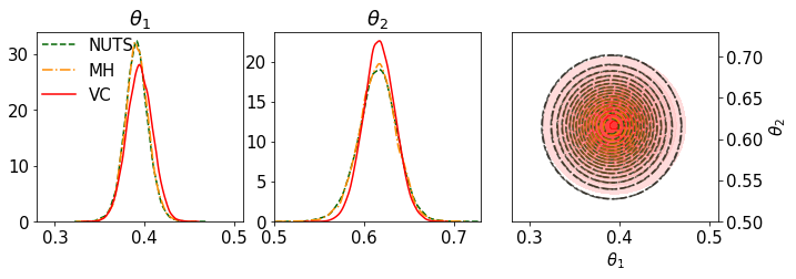
4.校准结果
#### Loading the
n_obs = 144
#n_vc = 22798
n_vc = 23000
n_steps = 150000
S = 50
l =3
#l =
vine_type = "D"
learning_rate = "AdaGrad"
eta = 0.07
decay = 1.0
folder = str(n_obs) + "_S_" + str(S) + "_l_" + str(l) + "_vine_" + vine_type + "_learning_" + learning_rate + \
                                    "_eta_" + str(eta) + "_decay_" + str(decay)
var_lambda_array = np.load("Simulation_results/Calibration/OBB_"  + folder + "/" + "param_nobs_" + str(n_obs) + "_S_" + str(S) + "_l_" + str(l) +  "_vine_" + vine_type + "_step_" + str(n_steps) +".npy")
tau_array = np.load("Simulation_results/Calibration/OBB_"  + folder + "/" + "tau_nobs_" + str(n_obs) + "_S_" + str(S) + "_l_" + str(l) +  "_vine_" + vine_type + "_step_" + str(n_steps) +".npy")
time_array = np.load("Simulation_results/Calibration/OBB_"  + folder + "/" + "time_nobs_" + str(n_obs) + "_S_" + str(S) + "_l_" + str(l) +  "_vine_" + vine_type + "_step_" + str(n_steps) +".npy")
mean_theta = var_lambda_array[-1,:2] # First two elements are the mean
cov_theta = np.log(np.exp(var_lambda_array[-1,2:4]) + 1) # 3-4 are the transformed standard deviations
dim = 2
theta_variational = theta_prior = gaussian_mean_field_family(param = {"mu": mean_theta, "sigma": cov_theta}, dim = dim)

fig = plt.figure(figsize=(11, 3.5))
plt.rcParams.update({'font.size': 15})
gs = gridspec.GridSpec(1, 3)
n_levels = 20
bw = 0.030
bins = 50
alpha = 0.8
shade = False

ax = []
ax = ax + [plt.subplot(gs[0])]
ax = ax + [plt.subplot(gs[1])]
ax = ax + [plt.subplot(gs[2])]
plt.subplots_adjust(wspace = 0.15)

sns.distplot(trace_NUTS['theta'][25000:,0], bins = bins, ax = ax[0], label = 'NUTS', hist =False, color = "darkgreen", kde_kws={'linestyle':'--'})
sns.distplot(trace['theta'][25000:,0], bins = bins, ax = ax[0], label = 'MH', hist = False, color = "darkorange", kde_kws={'linestyle':'-.'})
sns.distplot(theta_variational.sample(25000)[:,0], bins = bins, ax = ax[0], label = 'VC', hist = False, color = "red", kde_kws={'linestyle':'-'})
ax[0].legend(frameon=False, bbox_to_anchor=(-0.05,1.05),loc = "upper left")
ax[0].title.set_text(r'$\theta_1$')

sns.distplot(trace_NUTS['theta'][25000:,1], bins = bins, ax = ax[1], hist =False, color = "darkgreen", kde_kws={'linestyle':'--'})
sns.distplot(trace['theta'][25000:,1], bins = bins, ax = ax[1],  hist = False, color = "darkorange", kde_kws={'linestyle':'-.'})
sns.distplot(theta_variational.sample(25000)[:,1], bins = bins, ax = ax[1], hist = False, color = "red", kde_kws={'linestyle':'-'})
ax[1].title.set_text(r'$\theta_2$')

sns.kdeplot(trace_NUTS['theta'][25000:,0], trace_NUTS['theta'][25000:,1], ax=ax[2], n_levels=n_levels, shade=shade, shade_lowest=shade, alpha = alpha, bw = bw, color = "darkgreen", label = 'NUTS', linestyles = '--')
sns.kdeplot(theta_variational.sample(25000)[:,0], theta_variational.sample(25000)[:,1], ax=ax[2], n_levels=n_levels,shade=True, shade_lowest=False, alpha = alpha, bw = bw, color = "red", label = 'VC')
sns.kdeplot(trace['theta'][25000:,0], trace['theta'][25000:,1], ax=ax[2], n_levels=n_levels, shade=shade, shade_lowest=shade, alpha = alpha, bw = bw, color = "darkorange", label = 'MH', linestyles = '-.')
ax[2].set_xlabel(r'$\theta_1$')
ax[2].set_ylabel(r'$\theta_2$')
ax[2].yaxis.tick_right()
ax[2].yaxis.set_label_position("right")
#ax[2].legend(frameon=False)

#AX lims
ax[2].set_xlim([0.28, 0.51])
ax[2].set_ylim([0.5, 0.73])

ax[0].set_xlim([0.28, 0.51])
ax[1].set_xlim([0.5, 0.73])

plt.gcf().subplots_adjust(bottom=0.2)
plt.savefig("calibration_quality" + '.pdf', dpi=600)
plt.show()


 被折叠的 条评论
为什么被折叠?
被折叠的 条评论
为什么被折叠?
 到【灌水乐园】发言


