keras之Deep Learning with ConvNets

最新推荐文章于 2023-01-04 22:53:46 发布

yinfang1252

最新推荐文章于 2023-01-04 22:53:46 发布

阅读量855

点赞数

分类专栏： keras

keras 专栏收录该内容

4 篇文章 0 订阅

订阅专栏

CNN可以利用空间信息因此非常适合用来做图像分类。它的灵感来源于人的视觉皮层的数据处理过程。

1.深度CNN-DCNN

DCNN包含很多神经网络层，通常是由卷积层和池化层交替构成。从左至右网络层的filter的深度是在不断增加的，最后一层通常由一或多个连接层构成。

除了卷积层，还有三个关键的概念：

局部感受野
共享权重
池化层

1.1 局部感受野Local receptive fields

如果我们想要保存空间信息，那么用像素矩阵表示每幅图像是很方便的。那么，对局部结构进行编码的一个简单方法是将相邻输入神经元的子矩阵连接到属于下一层的单个隐神经元中。这个单个隐神经元代表一个局部感受野。注意，这个操作名为卷积，它给出了这种网络的名称。

当然，我们可以通过重叠的子矩阵来编码更多的信息。例如，假设每个子矩阵的大小为5x5，而这些子矩阵与28x28像素的mnist图像一起使用，那么我们就能够在下一个隐藏层生成23x23个局部感受区神经元。事实上，在触及图像的边界之前，只需将子矩阵滑动23个位置即可。在角点中，每个子矩阵的大小称为跨距长度(stride length)，这是一个在构建网络时可以进行精细调整的超参数。

让我们定义从一个层到另一个层的特征映射。当然，我们可以有多个特征映射，它们可以独立于每个隐藏层学习。例如，我们可以从28x28个输入神经元开始处理MInst图像，然后在下一个隐藏层中回忆每个23x23个神经元的k个特征映射(同样是5×5的步幅)。

1.2共享权重和偏差

让我们假设我们想要摆脱用一行（列）的像素表示，通过独立于输入图像中的位置来检测相同的特征。一个简单的直觉就是对隐藏层中的所有神经元使用相同的权重和偏差。这样，每一层将学习一组位置无关的潜在特征，这些特征是从图像中派生出来的。

权值共享就是用同一个filter去对整个图片进行扫描。更多请参照：知乎

假设输入图像在三个通道上具有TF(TensorFlow)顺序的形状(256，256)，则表示为(256，256，3)。

在Keras中，如果我们想要添加一个具有输出32的维数和每个滤波器3x3的扩展的卷积层，我们将写：

model = Sequential()
model.add(Conv2D(32, (3, 3), input_shape=(256, 256, 3))

也可以写做：

model = Sequential()
model.add(Conv2D(32, kernel_size=3, input_shape=(256, 256, 3))

这意味着我们要在一个三通道的256 x 256图像上应用3x3卷积，产生32个输出通道(或输出滤波器)

1.3池化层

让我们假设我们想要总结一个特征映射的输出。再次，我们可以利用单个特征映射产生的输出的空间连续性，并将子矩阵的值聚合成一个综合描述与该物理区域相关的意义的输出值

1.3.1Max-pooling

它只是输出区域中观察到的最大激活值：

model.add(MaxPooling2D(pool_size = (2, 2)))

1.3.2Average pooling

另一种选择是平均池，它仅将一个区域聚集到该区域所观察到的激活的平均值中

更多的可以自己去keras文档查看

1.4小结

到目前为止，我们已经描述了卷积的基本概念，CNNs在一维中对时间维的音频和文本数据应用卷积和池操作，在沿(高度x宽度)维度上的图像二维中使用卷积和池操作，在沿(高度x宽度x时间)维度上对视频进行三维卷积和池操作。

对于图像，滑动滤波器在输入体积上产生一个映射，给出滤波器对每个空间位置的响应。换句话说，ConvNet有多个滤波器叠加在一起，它们学习识别特定的视觉特征，而不依赖于图像中的位置。这些视觉特征在网络的初始层很简单，然后在网络中变得越来越复杂。

2.DCNN实例---LeNet

Yann le Cun 提出了一个CNN集合名为LeNet，它被用来识别手写数字，对于简单的几何变换和歪曲有着鲁棒性（Convolutional Networks for Images, Speech, and Time-Series, by Y. LeCun and Y. Bengio, brain theory neural networks, vol. 3361, 1995）。这里的关键步骤是有低层交替卷积操作和最大池操作，卷积运算是基于仔细选择的多特征映射的局部接收域，并具有共享权重。然后，更高层次是基于传统MLP的完全连接层，其中隐藏层是隐藏层，输出层是Softmax。

2.1LeNet code in Keras

为了定义lenet代码，我们使用了一个卷积2d模块，它是

keras.layers.convolutional.Conv2D(filters, kernel_size, padding='valid')

这里，filters是使用的卷积核数目，也是输出的维数。kernel_size是一个由两个整数组成的整数或元组/列表，指定2d卷积窗口的宽度和高度(可以是单个整数，用于为所有空间维度指定相同的值)。 padding='same'意味着使用填充。有两个选项：padding=‘Valid’意味着只有在输入和滤波器完全重叠的情况下才计算卷积，因此输出比输入小，而padding=‘same’则意味着我们有一个与输入相同大小的输出，输入周围的区域被填充为零。
另外，我们也是使用池化层：

keras.layers.pooling.MaxPooling2D(pool_size=(2, 2), strides=(2, 2))

Pool_size=(2，2)是一个由两个整数组成的元组，表示图像垂直和水平下降的因素，因此(2，2)将图像在每个维度减半，而strides=(2，2)是用于处理的步长。

接下来，我们来定义Lenet：

from keras import backend as K
from keras import Sequential
from keras.layers import Conv2D,MaxPooling2D,Activation
from keras.layers import Flatten,Dense
from keras.datasets import mnist
from keras.utils import np_utils
from keras.optimizers import SGD,RMSprop,Adam
import numpy as np
import matplotlib.pyplot as plt

#define the convnet
class LeNet:
    @staticmethod
    def bulid(input_shape,classes):
        model=Sequential()
        #conv--RELU--POOL
        model.add(Conv2D(20,(5,5),padding='same',input_shape=input_shape,activation='relu'))
        model.add(MaxPooling2D((2,2),(2,2)))
        #conv--RELU--POOL
        model.add(Conv2D(50,(5,5),border_mode='same',activation='relu'))
        model.add(MaxPooling2D((2,2),(2,2)))
        # Flatten => RELU layers
        model.add(Flatten())
        model.add(Dense(500,activation='relu'))
        # a softmax classifier
        model.add(Dense(classes,activation='softmax'))
        return model

结构如下所示

现在就是训练网络，查看损失了：

# network and training
NB_EPOCH = 20
BATCH_SIZE = 128
VERBOSE = 1
OPTIMIZER = Adam()
VALIDATION_SPLIT=0.2
IMG_ROWS, IMG_COLS = 28, 28 # input image dimensions
NB_CLASSES = 10 # number of outputs = number of digits
INPUT_SHAPE = (IMG_ROWS, IMG_COLS,1)#我使用的是tenorflow后端，通道数放在后面
# data: shuffled and split between train and test sets
(X_train, y_train), (X_test, y_test) = mnist.load_data()
# consider them as float and normalize
X_train = X_train.astype('float32')
X_test = X_test.astype('float32')
X_train /= 255
X_test /= 255
# we need a 60K x [1 x 28 x 28] shape as input to the CONVNET
X_train = X_train[:, :, :,np.newaxis]##这里注意新插的轴的位置
X_test = X_test[:,:, :,np.newaxis]
print(X_train.shape[0], 'train samples')
print(X_test.shape[0], 'test samples')
# convert class vectors to binary class matrices
y_train = np_utils.to_categorical(y_train, NB_CLASSES)
y_test = np_utils.to_categorical(y_test, NB_CLASSES)
# initialize the optimizer and model
model = LeNet.build(input_shape=INPUT_SHAPE, classes=NB_CLASSES)
model.compile(loss="categorical_crossentropy", optimizer=OPTIMIZER,metrics=["accuracy"])
history = model.fit(X_train, y_train,batch_size=BATCH_SIZE, epochs=NB_EPOCH,
                    verbose=VERBOSE, validation_split=VALIDATION_SPLIT)
score = model.evaluate(X_test, y_test, verbose=VERBOSE)
print("Test score:", score[0])
print('Test accuracy:', score[1])
# list all data in history
print(history.history.keys())
# summarize history for accuracy
plt.plot(history.history['acc'])
plt.plot(history.history['val_acc'])
plt.title('model accuracy')
plt.ylabel('accuracy')
plt.xlabel('epoch')
plt.legend(['train', 'test'], loc='upper left')
plt.show()
# summarize history for loss
plt.plot(history.history['loss'])
plt.plot(history.history['val_loss'])
plt.title('model loss')
plt.ylabel('loss')
plt.xlabel('epoch')
plt.legend(['train', 'test'], loc='upper left')
plt.show()

注意一下：使用tensorflow或者theano后端在输入维度上是不一致的。

输出结果如下：

60000 train samples
10000 test samples
E:/项目集合/兴趣项目/keras/Deep Learning with ConvNets/tt1.py:25: UserWarning: Update your `Conv2D` call to the Keras 2 API: `Conv2D(50, (5, 5), activation="relu", padding="same")`
  model.add(Conv2D(50,(5,5),border_mode='same',activation='relu'))
Train on 48000 samples, validate on 12000 samples
Epoch 1/20
48000/48000 [==============================] - 88s 2ms/step - loss: 0.1808 - acc: 0.9444 - val_loss: 0.0561 - val_acc: 0.9837
Epoch 2/20
48000/48000 [==============================] - 87s 2ms/step - loss: 0.0474 - acc: 0.9851 - val_loss: 0.0449 - val_acc: 0.9867
Epoch 3/20
48000/48000 [==============================] - 89s 2ms/step - loss: 0.0346 - acc: 0.9890 - val_loss: 0.0397 - val_acc: 0.9874
Epoch 4/20
48000/48000 [==============================] - 92s 2ms/step - loss: 0.0228 - acc: 0.9925 - val_loss: 0.0356 - val_acc: 0.9895
Epoch 5/20
48000/48000 [==============================] - 93s 2ms/step - loss: 0.0169 - acc: 0.9946 - val_loss: 0.0379 - val_acc: 0.9892
Epoch 6/20
48000/48000 [==============================] - 84s 2ms/step - loss: 0.0133 - acc: 0.9954 - val_loss: 0.0379 - val_acc: 0.9892
Epoch 7/20
48000/48000 [==============================] - 88s 2ms/step - loss: 0.0118 - acc: 0.9961 - val_loss: 0.0299 - val_acc: 0.9922
Epoch 8/20
48000/48000 [==============================] - 84s 2ms/step - loss: 0.0090 - acc: 0.9971 - val_loss: 0.0344 - val_acc: 0.9910
Epoch 9/20
48000/48000 [==============================] - 83s 2ms/step - loss: 0.0065 - acc: 0.9977 - val_loss: 0.0592 - val_acc: 0.9864
Epoch 10/20
48000/48000 [==============================] - 83s 2ms/step - loss: 0.0072 - acc: 0.9977 - val_loss: 0.0369 - val_acc: 0.9915
Epoch 11/20
48000/48000 [==============================] - 83s 2ms/step - loss: 0.0050 - acc: 0.9983 - val_loss: 0.0371 - val_acc: 0.9923
Epoch 12/20
48000/48000 [==============================] - 82s 2ms/step - loss: 0.0066 - acc: 0.9976 - val_loss: 0.0428 - val_acc: 0.9902
Epoch 13/20
48000/48000 [==============================] - 83s 2ms/step - loss: 0.0051 - acc: 0.9984 - val_loss: 0.0501 - val_acc: 0.9889
Epoch 14/20
48000/48000 [==============================] - 84s 2ms/step - loss: 0.0034 - acc: 0.9989 - val_loss: 0.0384 - val_acc: 0.9922
Epoch 15/20
48000/48000 [==============================] - 85s 2ms/step - loss: 0.0063 - acc: 0.9980 - val_loss: 0.0415 - val_acc: 0.9910
Epoch 16/20
48000/48000 [==============================] - 83s 2ms/step - loss: 0.0049 - acc: 0.9984 - val_loss: 0.0425 - val_acc: 0.9917
Epoch 17/20
48000/48000 [==============================] - 83s 2ms/step - loss: 0.0045 - acc: 0.9987 - val_loss: 0.0434 - val_acc: 0.9923
Epoch 18/20
48000/48000 [==============================] - 85s 2ms/step - loss: 0.0016 - acc: 0.9994 - val_loss: 0.0517 - val_acc: 0.9907
Epoch 19/20
48000/48000 [==============================] - 85s 2ms/step - loss: 0.0069 - acc: 0.9976 - val_loss: 0.0401 - val_acc: 0.9916
Epoch 20/20
48000/48000 [==============================] - 88s 2ms/step - loss: 0.0039 - acc: 0.9988 - val_loss: 0.0431 - val_acc: 0.9902
10000/10000 [==============================] - 6s 594us/step
Test score: 0.03449039720774735
Test accuracy: 0.9917
dict_keys(['val_loss', 'val_acc', 'loss', 'acc'])

2.2Understanding the power of deep learning

可以看到，深度网络的性能总是好于浅的网络，当数据集规模越小时，差距越大。从数学的角度看，这可能令人惊讶，因为深层网络有更多的未知(权重)，因此人们会认为我们需要更多的数据点。然而，保存空间信息、添加卷积、池和特征映射是卷积网的创新。

3.Recognizing CIFAR-10 images with deep learning

CIFAR-10数据集包含60000张彩色的32*32的三通道图片，并被划分为10类，每类包含6000张图片。train set包含50000张，test set 包含10000张。实例如下。更多信息可以百度

首先尝试一下简单模型：

from keras.datasets import cifar10
from keras.utils import np_utils
from keras.models import Sequential
from keras.layers.core import Dense, Dropout, Activation, Flatten
from keras.layers.convolutional import Conv2D, MaxPooling2D
from keras.optimizers import SGD, Adam, RMSprop
import matplotlib.pyplot as plt

#定义input data的信息
IMG_CHANNELS=3
IMG_ROWS=32
IMG_COLS=32

#定义常量
BATCH_SIZE=128
NB_EPOCH=20
NB_CLASSES=10
VERBOSE=1#日志显示，0为不在标准输出流输出日志信息，1为输出进度条记录，2为每个epoch输出一行记录
VALIDATION_SPLIT = 0.2
OPTIM=RMSprop()

#load the dataset
(X_train, y_train), (X_test, y_test) = cifar10.load_data()
print('X_train shape:', X_train.shape)
print(X_train.shape[0], 'train samples')
print(X_test.shape[0], 'test samples')

# convert to categorical
Y_train = np_utils.to_categorical(y_train, NB_CLASSES)
Y_test = np_utils.to_categorical(y_test, NB_CLASSES)

# float and normalization
X_train = X_train.astype('float32')
X_test = X_test.astype('float32')
X_train /= 255
X_test /= 255

##network
model = Sequential()
#第一层与input的维度一致，是为了引入非线性
model.add(Conv2D(32, (3, 3), padding='same',
                 input_shape=(IMG_ROWS, IMG_COLS, IMG_CHANNELS)))
model.add(Activation('relu'))
model.add(MaxPooling2D(pool_size=(2, 2)))
model.add(Dropout(0.25))
model.add(Flatten())
model.add(Dense(512))
model.add(Activation('relu'))
model.add(Dropout(0.5))
model.add(Dense(NB_CLASSES))
model.add(Activation('softmax'))
model.summary()


# train
model.compile(loss='categorical_crossentropy', optimizer=OPTIM,
metrics=['accuracy'])
model.fit(X_train, Y_train, batch_size=BATCH_SIZE,
          epochs=NB_EPOCH, validation_split=VALIDATION_SPLIT,verbose=VERBOSE)
score = model.evaluate(X_test, Y_test,batch_size=BATCH_SIZE, verbose=VERBOSE)
print("Test score:", score[0])
print('Test accuracy:', score[1])

#save model
model_json = model.to_json()
open('cifar10_architecture.json', 'w').write(model_json)
#And the weights learned by our deep network on the training set
model.save_weights('cifar10_weights.h5', overwrite=True)

上面的网络很简单，也就是conv--maxpool--dropout--flatten--dense--dropout--softmax

最后测试正确率大约在66.4%左右（20次迭代）

3.1Improving the CIFAR-10 performance with deeper a network

上一节也提过，加深网络层可以提高网络性能，这一小节，我们将模型加深为以下格式：

conv+conv+maxpool+dropout+conv+conv+maxpool+dense+dropout+dense

也就是将模型那一块改为：

model = Sequential()
model.add(Conv2D(32, (3, 3), padding='same',input_shape=(IMG_ROWS, IMG_COLS, IMG_CHANNELS)))
model.add(Activation('relu'))
model.add(Conv2D(32, (3, 3), padding='same'))
model.add(Activation('relu'))
model.add(MaxPooling2D(pool_size=(2, 2)))
model.add(Dropout(0.25))
model.add(Conv2D(64, (3, 3), padding='same'))
model.add(Activation('relu'))
model.add(Conv2D(64, 3, 3))
model.add(Activation('relu'))
model.add(MaxPooling2D(pool_size=(2, 2)))
model.add(Dropout(0.25))
model.add(Flatten())
model.add(Dense(512))
model.add(Activation('relu'))
model.add(Dropout(0.5))
model.add(Dense(NB_CLASSES))
model.add(Activation('softmax'))

迭代40次正确率可以达到76.9%，显著提高。

3.2Improving the CIFAR-10 performance with data
augmentation

一种提高性能的方法是为我们的培训生成更多的图像。关键的直觉是我们可以采用标准的CIFAR培训集，并通过多种类型的转换来增强这个集合，包括旋转、重标、水平/垂直翻转、缩放、信道移位等等。

from keras.preprocessing.image import ImageDataGenerator
from keras.datasets import cifar10
import numpy as np
NUM_TO_AUGMENT=5
#load dataset
(X_train, y_train), (X_test, y_test) = cifar10.load_data()
# augumenting
print("Augmenting training set images...")
datagen = ImageDataGenerator(
    rotation_range=40,
    width_shift_range=0.2,
    height_shift_range=0.2,
    zoom_range=0.2,
    horizontal_flip=True,
    fill_mode='nearest')

rotation_range 是随机旋转图片的度数(0-180)。width_shift 和 height_shift是用于垂直或水平地随机转换图片的范围。zoom_range用于随机缩放图片。horizontal_flip用于随机翻转一半图像水平。 fill_mode是用于填充旋转或移位后可能出现的新像素的策略。

xtas, ytas = [], []
for i in range(X_train.shape[0]):
    num_aug = 0
    x = X_train[i] # (3, 32, 32)
    x = x.reshape((1,) + x.shape) # (1, 3, 32, 32)
    for x_aug in datagen.flow(x, batch_size=1,
        save_to_dir='preview', save_prefix='cifar', save_format='jpeg'):
        if num_aug >= NUM_TO_AUGMENT:
            break
        xtas.append(x_aug[0])
    num_aug += 1

现在，我们可以直接将这种直觉应用于培训。使用前面定义的相同的ConvNet，我们只需生成更多的增强图像，然后我们就可以进行培训。为了提高效率，生成器与模型并行运行。这允许在CPU上进行图像增强，并与gpus上的培训并行。下面是代码

#fit the dataget
datagen.fit(X_train)
# train
history = model.fit_generator(datagen.flow(X_train, Y_train,
    batch_size=BATCH_SIZE), samples_per_epoch=X_train.shape[0],
    epochs=NB_EPOCH, verbose=VERBOSE)
    score = model.evaluate(X_test, Y_test,
    batch_size=BATCH_SIZE, verbose=VERBOSE)
print("Test score:", score[0])
print('Test accuracy:', score[1])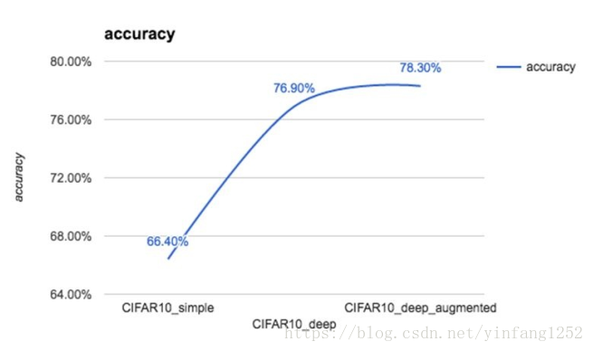

3.3Predicting with CIFAR-10

import numpy as np
import scipy.misc
from keras.models import model_from_json
from keras.optimizers import SGD
#load model
model_architecture = 'cifar10_architecture.json'
model_weights = 'cifar10_weights.h5'
model = model_from_json(open(model_architecture).read())
model.load_weights(model_weights)
#load images
img_names = ['cat-standing.jpg', 'dog.jpg']
imgs = [np.transpose(scipy.misc.imresize(scipy.misc.imread(img_name), (32, 32)),
(1, 0, 2)).astype('float32') for img_name in img_names]
imgs = np.array(imgs) / 255
# train
optim = SGD()
model.compile(loss='categorical_crossentropy', optimizer=optim,metrics=['accuracy'])
# predict
predictions = model.predict_classes(imgs)
print(predictions)

4.Very deep convolutional networks for large-scale
image recognition

2014年一篇文章（Very Deep Convolutional Networks for Large-Scale Image Recognition, by K. Simonyan and A.
Zisserman, 2014）指出：通过将网络深度推进到16-19层，可以实现对现有技术配置的显著改进。

论文中所提到的网络就是VGG16,原文以caffe实现。用在ILSVRC-2012数据集上。这场竞赛的目的是评估照片的内容，以便使用大量手工标记的ImageNet数据集(1000万张标有10，000个对象类别的标记图像)的子集进行检索和自动标注。测试图像将不带初始注释--没有分割或标签--而算法必须生成标记，指定图像中存在哪些对象。

在caffe中实现的模型所学习的权重已直接转换为Keras（ https://gist.github.com/baraldilorenzo/07d7802847aaad0a35d3），可以用来预压到keras模型中。下面我们看一下VGG16模型：

from keras.models import Sequential
from keras.layers.core import Flatten, Dense, Dropout
from keras.layers.convolutional import Conv2D, MaxPooling2D, ZeroPadding2D
from keras.optimizers import SGD
import cv2, numpy as np

def VGG_16(weights_path=None):
    model = Sequential()
    model.add(ZeroPadding2D((1,1),input_shape=(3,224,224)))
    model.add(Conv2D(64, (3, 3), activation='relu'))
    model.add(ZeroPadding2D((1,1)))
    model.add(Conv2D(64, (3, 3), activation='relu'))
    model.add(MaxPooling2D((2,2), strides=(2,2)))
    model.add(ZeroPadding2D((1,1)))
    model.add(Conv2D(128, (3, 3), activation='relu'))
    model.add(ZeroPadding2D((1,1)))
    model.add(Conv2D(128, (3, 3), activation='relu'))
    model.add(MaxPooling2D((2,2), strides=(2,2)))
    model.add(ZeroPadding2D((1,1)))
    model.add(Conv2D(256, (3, 3), activation='relu'))
    model.add(ZeroPadding2D((1,1)))
    model.add(Conv2D(256, (3, 3), activation='relu'))
    model.add(ZeroPadding2D((1,1)))
    model.add(Conv2D(256, (3, 3), activation='relu'))
    model.add(MaxPooling2D((2,2), strides=(2,2)))
    model.add(ZeroPadding2D((1,1)))
    model.add(Conv2D(512, (3, 3), activation='relu'))
    model.add(ZeroPadding2D((1,1)))
    model.add(Conv2D(512, (3, 3), activation='relu'))
    model.add(ZeroPadding2D((1,1)))
    model.add(Conv2D(512, (3, 3), activation='relu'))
    model.add(MaxPooling2D((2,2), strides=(2,2)))
    model.add(ZeroPadding2D((1,1)))
    model.add(Conv2D(512, (3, 3), activation='relu'))
    model.add(ZeroPadding2D((1,1)))
    model.add(Conv2D(512, (3, 3), activation='relu'))
    model.add(ZeroPadding2D((1,1)))
    model.add(Conv2D(512, (3, 3), activation='relu'))
    model.add(MaxPooling2D((2,2), strides=(2,2)))
    model.add(Flatten())
    #top layer of the VGG net
    model.add(Dense(4096, activation='relu'))
    model.add(Dropout(0.5))
    model.add(Dense(4096, activation='relu'))
    model.add(Dropout(0.5))
    model.add(Dense(1000, activation='softmax'))
    if weights_path:
    model.load_weights(weights_path)
    return model

4.1使用VGG16网络识别猫

im = cv2.resize(cv2.imread('cat.jpg'), (224, 224)).astype(np.float32)
im = im.transpose((2,0,1))
im = np.expand_dims(im, axis=0)
# Test pretrained model
model = VGG_16('/Users/gulli/Keras/codeBook/code/data/vgg16_weights.h5')
optimizer = SGD()
model.compile(optimizer=optimizer, loss='categorical_crossentropy')
out = model.predict(im)
print np.argmax(out)

这儿是从原书直接copy的源代码，没有下载预权重，所以就不展示结果了。

4.2使用keras模块构建VGG16

Keras预先构建和训练了很多深度学习模型。在实例化模型时自动下载权重，并存储在~/.keras/model/。使用内置代码非常容易。

from keras.models import Model
from keras.preprocessing import image
from keras.optimizers import SGD
from keras.applications.vgg16 import VGG16
import matplotlib.pyplot as plt
import numpy as np
import cv2
# prebuild model with pre-trained weights on imagenet
model = VGG16(weights='imagenet', include_top=True)
sgd = SGD(lr=0.1, decay=1e-6, momentum=0.9, nesterov=True)
model.compile(optimizer=sgd, loss='categorical_crossentropy')
# resize into VGG16 trained images' format
im = cv2.resize(cv2.imread('steam-locomotive.jpg'), (224, 224))
im = np.expand_dims(im, axis=0)
# predict
out = model.predict(im)
plt.plot(out.ravel())
plt.show()
print np.argmax(out)
#this should print 820 for steaming trai

4.3

迁移学习是一种非常强大的深度学习技术，在不同的领域有更多的应用。直觉非常简单，可以用类比来解释。假设你想学习一门新语言，比如说西班牙语；那么从你已经知道的语言(比如英语)开始是非常有用的。