tensorflow 11：双隐层+softmax回归实现mnist图片识别

最新推荐文章于 2023-03-02 09:30:51 发布

yuanlulu

最新推荐文章于 2023-03-02 09:30:51 发布

阅读量3k

点赞数

分类专栏： python tensorflow案例：一步一个脚印

本文链接：https://blog.csdn.net/yuanlulu/article/details/82952436

版权

DL/ML/AI 同时被 3 个专栏收录

88 篇文章 5 订阅

订阅专栏

python

65 篇文章 4 订阅

订阅专栏

机器学习

59 篇文章 6 订阅

订阅专栏

概述

上篇文章讲到的sofmax回归，除了输入层，只有线性层+sofmax,这两者合起来可以被称为输出层。没有中间的隐藏层。

本文介绍在sofmax回归基础上增加两层隐藏层的方法。

本文的主要参考来自参考资料里的《TensorFlow运作方式入门》和《TensorFlow实现双隐层SoftMax Regression分类器》。

主要代码来自tensorflow源码目录下的例程mnist.py。

借用别人的一张图，双隐藏层的结构如下：
在这里插入图片描述

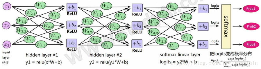
注意上图W和b的下标是不对的，出处的作者也是偷懒，粘贴拷贝组合成的新图。

构建计算图的过程

参考前篇文章，构建一个计算图需要4个阶段：

Inference:构建前向预测节点
Loss:构建损失节点
Train:构建训练节点
Evaluate: 构建评估节点

tensorflow自带例程tensorflow/examples/tutorials/mnist/mnist.py，里面实现了上述4个阶段，并且每个阶段抽象为一个函数。原始的文件是给同一目录下的另一个文件fully_connected_feed.py调用的。本文修改了mnist.py使之可独立运行，没有牵扯到fully_connected_feed.py。

构建模型计算图讲解

推理（Inference）

inference()函数会尽可能地构建图表，最终返回包含了预测结果（output prediction）的Tensor。
本阶段需要构建两个隐藏层和一个“线性+softmax回归层”。

每一层都创建于一个唯一的tf.name_scope之下，创建于该作用域之下的所有元素都将带有其前缀。

with tf.name_scope('hidden2'):

在定义的作用域中，每一层所使用的权重和偏差都在使用tf.Variable生成，并且包含了各自期望的shape。

weights = tf.Variable(
        tf.truncated_normal([hidden1_units, hidden2_units],
                            stddev=1.0 / math.sqrt(float(hidden1_units))),
                            name='weights')
biases = tf.Variable(tf.zeros([hidden2_units]), name='biases')

当这些层是在hidden2作用域下生成时，赋予权重变量的独特名称将会是"hidden2/weights".

通过tf.truncated_normal函数初始化权重变量, tf.truncated_normal初始函数将根据所得到的均值和标准差，生成一个随机分布。

多说一句 tf.truncated_normal，这个函数是一种截断正太分布初始化，也就是说它赋给变量的值的范围不是无穷大，而是默认在两倍标准差的范围内。

然后，通过tf.zeros函数初始化偏差变量（biases），确保所有偏差的起始值都是0，而它们的shape则是其在该层中所接到的（connect to）单元数量。

其中两个隐藏层后面还有一个Relu激活函数：

hidden2 = tf.nn.relu(tf.matmul(hidden1, weights) + biases)

输出层没有激活函数。输出结果在做loss计算时用tf.nn.sparse_softmax_cross_entropy_with_logits做softmax计算。

推理构造函数返回的是输出层最后输出的tensor。

损失（Loss）

loss()函数通过添加所需的损失操作，进一步构建图表。

添加一个tf.nn.softmax_cross_entropy_with_logits操作，用来比较inference()函数所输出的logits Tensor softmax之后和lable的交叉熵，然后求平均值。

cross_entropy = tf.nn.sparse_softmax_cross_entropy_with_logits(
      labels=labels, logits=logits, name='xentropy')
return tf.reduce_mean(cross_entropy, name='xentropy_mean')

训练（Train）

training()函数添加了通过梯度下降（gradient descent）将损失最小化所需的操作。

实例化一个tf.train.GradientDescentOptimizer，负责按照所要求的学习效率（learning rate）应用梯度下降法（gradients），并使用minimize()函数更新系统中的权重，不断地修改变量以降低成本。

# 根据给定的学习率创建梯度下降优化器
optimizer = tf.train.GradientDescentOptimizer(learning_rate)
train_op = optimizer.minimize(loss=loss,global_step=global_step)

另外，为了能够在tensorboard可视化训练过程，还增加了loss的汇总值，并在minimize过程中不断更新global_step。

# 为保存loss的值添加一个标量汇总(scalar summary).
tf.summary.scalar('loss', loss)

# 创建一个变量来跟踪global step.
global_step = tf.Variable(0, name='global_step', trainable=False)

注意上面两端代码顺序是打乱的，为了分开表述才分开的，完整版看下面。

评估（Evaluate）

计算每个批次样本top-k结果的准确性（这里取top1），并累计预测正确的样本数量。

  correct = tf.nn.in_top_k(logits, labels, 1)

  # 返回 当前批次的样本中预测正确的样本数量.
  return tf.reduce_sum(tf.cast(correct, tf.int32))

循环训练模型

上述工作做完，就很容易得到各个模块的tensor，使之在session中run起来，提供正确的参数就可以了。

for step in range(1, num_steps+1):
    batch_x, batch_y = mnist.train.next_batch(batch_size)
    # Run optimization op (backprop)
    sess.run(train_op, feed_dict={images_placeholder: batch_x, labels_placeholder: batch_y})

每到一定的部署，调用一次loss和Evaluate节点评估当前的效果：

    if step % display_step == 0 or step == 1:
        # Calculate batch loss and accuracy
        loss, acc = sess.run([batch_loss, correct_counts], feed_dict={images_placeholder: batch_x, labels_placeholder: batch_y})
        print("Step " + str(step) + ", Minibatch Loss= " + \
              "{:.4f}".format(loss) + ", Training Accuracy= " + \
              "{:.3f}".format(float(acc)/batch_size))

所有训练做完以后，还要在测试集上测试最终的效果：

test_acc = sess.run(correct_counts, feed_dict={images_placeholder: mnist.test.images,
                                                labels_placeholder: mnist.test.labels})
print("Testing Accuracy:{:.3f}".format(float(test_acc)/len(mnist.test.images)))

完整代码

import math

import tensorflow as tf

# MNIST 有10个类, 表达了0到9的10个数字.
NUM_CLASSES = 10
# MNIST 中的图像都是 28x28 像素，展开成784维的特征向量
IMAGE_SIZE = 28
IMAGE_PIXELS = IMAGE_SIZE * IMAGE_SIZE
batch_size = 50 #每个批次的样本数量
hidden1_units = 20 #第一个隐藏层的大小.
hidden2_units = 15 #第二个隐藏层的大小.
learning_rate = 0.1 #优化器的学习率

images_placeholder = tf.placeholder(tf.float32, shape=(None, IMAGE_PIXELS))
labels_placeholder = tf.placeholder(tf.int32, shape=(None))

#构建学习器模型的前向预测过程(从输入到预测输出的计算图路径)
def inference(images, hidden1_units, hidden2_units):
  # Hidden 1：y1 = relu(x*W1 +b1)
  with tf.name_scope('hidden1'):
    weights = tf.Variable(
        tf.truncated_normal([IMAGE_PIXELS, hidden1_units],
                            stddev=1.0 / math.sqrt(float(IMAGE_PIXELS))),
                            name='weights')
    biases = tf.Variable(tf.zeros([hidden1_units]), name='biases')
    hidden1 = tf.nn.relu(tf.matmul(images, weights) + biases)
  # Hidden 2: y2 = relu(y1*W2 + b2)
  with tf.name_scope('hidden2'):
    weights = tf.Variable(
        tf.truncated_normal([hidden1_units, hidden2_units],
                            stddev=1.0 / math.sqrt(float(hidden1_units))),
                            name='weights')
    biases = tf.Variable(tf.zeros([hidden2_units]), name='biases')
    hidden2 = tf.nn.relu(tf.matmul(hidden1, weights) + biases)
  # Linear: logits = y2*W3 + b3
  with tf.name_scope('softmax_linear'):
    weights = tf.Variable(
        tf.truncated_normal([hidden2_units, NUM_CLASSES],
                            stddev=1.0 / math.sqrt(float(hidden2_units))),
                            name='weights')
    biases = tf.Variable(tf.zeros([NUM_CLASSES]), name='biases')
    logits = tf.matmul(hidden2, weights) + biases
  return logits

#根据logits和labels计算输出层损失。
def loss(logits, labels):
  labels = tf.to_int64(labels)
  cross_entropy = tf.nn.sparse_softmax_cross_entropy_with_logits(
      labels=labels, logits=logits, name='xentropy')
  return tf.reduce_mean(cross_entropy, name='xentropy_mean')

#为损失模型添加训练节点(需要产生和应用梯度的节点)
def training(loss, learning_rate):
  # 为保存loss的值添加一个标量汇总(scalar summary).
  tf.summary.scalar('loss', loss)
  # 根据给定的学习率创建梯度下降优化器
  optimizer = tf.train.GradientDescentOptimizer(learning_rate)
  # 创建一个变量来跟踪global step.
  global_step = tf.Variable(0, name='global_step', trainable=False)
  # 在训练节点，使用optimizer将梯度下降法应用到可调参数上来最小化损失
  # (同时不断增加 global step 计数器) .
  train_op = optimizer.minimize(loss=loss,global_step=global_step)
  return train_op

#评估模型输出的logits在预测类标签方面的质量
def evaluation(logits, labels):
  correct = tf.nn.in_top_k(logits, labels, 1)

  # 返回 当前批次的样本中预测正确的样本数量.
  return tf.reduce_sum(tf.cast(correct, tf.int32))

if __name__ == '__main__':
    num_steps = 5000
    display_step = 200

    # Import MNIST data
    from tensorflow.examples.tutorials.mnist import input_data

    mnist = input_data.read_data_sets( "./data/" )

    logits = inference(images_placeholder,hidden1_units, hidden2_units)

    batch_loss = loss(logits=logits, labels=labels_placeholder)

    train_op = training(loss=batch_loss, learning_rate=learning_rate)

    correct_counts =  evaluation(logits=logits, labels=labels_placeholder)

    ##调用Summary.FileWriter写入计算图
    writer = tf.summary.FileWriter("logs/mnistboard", tf.get_default_graph())
    writer.close()

    # Initialize the variables (i.e. assign their default value)
    init = tf.global_variables_initializer()

    # Start training
    with tf.Session() as sess:

        # Run the initializer
        sess.run(init)

        for step in range(1, num_steps+1):
            batch_x, batch_y = mnist.train.next_batch(batch_size)
            # Run optimization op (backprop)
            sess.run(train_op, feed_dict={images_placeholder: batch_x, labels_placeholder: batch_y})
            if step % display_step == 0 or step == 1:
                # Calculate batch loss and accuracy
                loss, acc = sess.run([batch_loss, correct_counts], feed_dict={images_placeholder: batch_x, labels_placeholder: batch_y})
                print("Step " + str(step) + ", Minibatch Loss= " + \
                      "{:.4f}".format(loss) + ", Training Accuracy= " + \
                      "{:.3f}".format(float(acc)/batch_size))

        print("Optimization Finished!")

        # Calculate accuracy for MNIST test image
        test_acc = sess.run(correct_counts, feed_dict={images_placeholder: mnist.test.images,
                                                labels_placeholder: mnist.test.labels})
        print("Testing Accuracy:{:.3f}".format(float(test_acc)/len(mnist.test.images)))

测试结果

隐藏层1节点数	隐藏层2节点数	训练步数	测试集上的准确率
1000	1000	5000	0.977
100	100	5000	0.969
50	40	5000	0.964
50	40	2500	0.956
20	15	2500	0.937
20	15	500	0.907
20	15	5000	0.954

可以看到隐藏层节点不需要太多，50足矣。训练步数足够，就能达到很不错的效果。

另一种实现双隐层softmax回归的方法

在github上有个很出名的tensorflow例程项目TensorFlow-Examples，里面也有一个实现实现双隐层softmax回归的方法。这种方法相当简洁。

主要思想与上面的一致，就不详细说了。原版的代码因为隐层节点太多，batchsize大，训练步数少，最终准确率只有0.3。改过参数值以后，效果和上面的就接近了。所以说调参调参，还是有效果的。

""" Neural Network.

A 2-Hidden Layers Fully Connected Neural Network (a.k.a Multilayer Perceptron)
implementation with TensorFlow. This example is using the MNIST database
of handwritten digits (http://yann.lecun.com/exdb/mnist/).

Links:
    [MNIST Dataset](http://yann.lecun.com/exdb/mnist/).

Author: Aymeric Damien
Project: https://github.com/aymericdamien/TensorFlow-Examples/
"""

from __future__ import print_function

# Import MNIST data
from tensorflow.examples.tutorials.mnist import input_data
mnist = input_data.read_data_sets("./data/", one_hot=True)

import tensorflow as tf

# Parameters
learning_rate = 0.1
num_steps = 2500
batch_size = 50
display_step = 100

# Network Parameters
n_hidden_1 = 50 # 1st layer number of neurons
n_hidden_2 = 40 # 2nd layer number of neurons

num_input = 784 # MNIST data input (img shape: 28*28)
num_classes = 10 # MNIST total classes (0-9 digits)

# tf Graph input
X = tf.placeholder("float", [None, num_input])
Y = tf.placeholder("float", [None, num_classes])

# Store layers weight & bias
weights = {
    'h1': tf.Variable(tf.random_normal([num_input, n_hidden_1])),
    'h2': tf.Variable(tf.random_normal([n_hidden_1, n_hidden_2])),
    'out': tf.Variable(tf.random_normal([n_hidden_2, num_classes]))
}
biases = {
    'b1': tf.Variable(tf.random_normal([n_hidden_1])),
    'b2': tf.Variable(tf.random_normal([n_hidden_2])),
    'out': tf.Variable(tf.random_normal([num_classes]))
}


# Create model
def neural_net(x):
    # Hidden fully connected layer with 256 neurons
    #layer_1 = tf.add(tf.matmul(x, weights['h1']), biases['b1'])
    # Hidden fully connected layer with 256 neurons
    #layer_2 = tf.add(tf.matmul(layer_1, weights['h2']), biases['b2'])

    layer_1 = tf.nn.relu(tf.add(tf.matmul(x, weights['h1']), biases['b1']))
    layer_2 = tf.nn.relu(tf.add(tf.matmul(layer_1, weights['h2']), biases['b2']))

    # Output fully connected layer with a neuron for each class
    out_layer = tf.matmul(layer_2, weights['out']) + biases['out']
    return out_layer

# Construct model
logits = neural_net(X)
prediction = tf.nn.softmax(logits)

# Define loss and optimizer
loss_op = tf.reduce_mean(tf.nn.softmax_cross_entropy_with_logits(
    logits=logits, labels=Y))
optimizer = tf.train.AdamOptimizer(learning_rate=learning_rate)
train_op = optimizer.minimize(loss_op)

# Evaluate model
correct_pred = tf.equal(tf.argmax(prediction, 1), tf.argmax(Y, 1))
accuracy = tf.reduce_mean(tf.cast(correct_pred, tf.float32))

# Initialize the variables (i.e. assign their default value)
init = tf.global_variables_initializer()

# Start training
with tf.Session() as sess:

    # Run the initializer
    sess.run(init)

    for step in range(1, num_steps+1):
        batch_x, batch_y = mnist.train.next_batch(batch_size)
        # Run optimization op (backprop)
        sess.run(train_op, feed_dict={X: batch_x, Y: batch_y})
        if step % display_step == 0 or step == 1:
            # Calculate batch loss and accuracy
            loss, acc = sess.run([loss_op, accuracy], feed_dict={X: batch_x,
                                                                 Y: batch_y})
            print("Step " + str(step) + ", Minibatch Loss= " + \
                  "{:.4f}".format(loss) + ", Training Accuracy= " + \
                  "{:.3f}".format(acc/batch_size))

    print("Optimization Finished!")

    # Calculate accuracy for MNIST test images
    print("Testing Accuracy:", \
        sess.run(accuracy, feed_dict={X: mnist.test.images,
                                      Y: mnist.test.labels}))

参考资料

tensorflow官方教程中文翻译：TensorFlow运作方式入门

TensorFlow实现双隐层SoftMax Regression分类器

TensorFlow-Examples/examples/3_NeuralNetworks/neural_network_raw.py

yuanlulu

关注

0
点赞
踩
5

收藏

觉得还不错? 一键收藏
0
评论
tensorflow 11：双隐层+softmax回归实现mnist图片识别

概述上篇文章讲到的sofmax回归，除了输入层，只有线性层+sofmax,这两者合起来可以被称为输出层。没有中间的隐藏层。本文介绍在sofmax回归基础上增加两层隐藏层的方法。本文的主要参考来自参考资料里的《TensorFlow运作方式入门》和《TensorFlow实现双隐层SoftMax Regression分类器》。主要代码来自tensorflow源码目录下的例程mnist.py。借...
复制链接

扫一扫