Beta函数与Gamma函数及其与Beta分布的关系

相关函数在scipy.special

import scipy.special as ss
ss.beta(x1, x2)
 
 
1
2
 
 
1
2

相关分布（概率密度）在scipy.stats

import scipy.stats as st
ss.beta(a, b)           # 随机变量
 
 
1
2
 
 
1
2

β  Function：

B(x,y)=∫10tx−1(1−t)y−1dt

主要性质： 

B(x,y)=B(y,x)B(x,y)=(x−1)!(y−1)!(x+y−1)!

Γ  function

Γ(x)=∫∞0tx−1e−tdt

其递归形式如下： 

Γ(x+1)=xΓ(x)

关系

B(x,y)=Γ(x)Γ(y)Γ(x+y)

scipy中的相关实现

>>> from scipy.special import beta
>>> from scipy.special import gamma
>>> beta(6, 7) == gamma(6)*gamma(7)/gamma(6+7)
True
 
 
1
2
3
4
 
 
1
2
3
4

Beta distribution 及其与Beta function and Gamma function的关系

Beta分布的概率密度函数（pdf）为： 

f(x;α,β)===C⋅xα−1(1−x)β−1Γ(x+y)Γ(x)Γ(y)xα−1(1−x)β−11Beta(x,y)xα−1(1−x)β−1

f(x;2,2)=x(1−x)Beta(2,2)

>>> st.beta(2, 2).pdf(.5) == .5*.5/ss.beta(2, 2)
True
 
 
1
2
 
 
1
2

beta distribution是一种在[0, 1]区间上的连续分布，在[0, 1]区间内概率密度值可以为  ∞ ，再次证明了概率密度函数值不是密度。

import numpy as np
import scipy.special as ss
from scipy import integrate
import matplotlib.pyplot as plt

def beta(x, a, b):
    return x**(a-1)*(1-x)**(b-1)/ss.beta(a, b)

def show_pdf():
    x = np.arange(0, 1, .01)
    for (a, b) in [(.5, .5), (5, 1), (1, 3), (2, 2), (2, 5)]:
        plt.plot(x, beta_pdf(x, a, b), label='a={:.1f}, b={:.1f}'.format(a, b), lw=2)
    plt.legend(loc='upper center', frameon=False)
    plt.ylim([0, 3.5])
    plt.ylabel('pdf')
    plt.savefig('./imgs/pdf.png')
    plt.show()

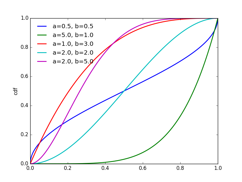
def show_cdf():
    x = np.arange(0+0.0001, 1, .0001)
    for (a, b) in [(.5, .5), (5, 1), (1, 3), (2, 2), (2, 5)]:
        plt.plot(x, [(integrate.quad(beta_pdf, 0, x, args=(a, b)))[0] for x in x],
                 label='a={:.1f}, b={:.1f}'.format(a, b), lw=2)
    plt.legend(loc='upper left', frameon=False)
    plt.ylabel('cdf')
    plt.savefig('./imgs/cdf.png')
    plt.show()

if __name__ == '__main__':
    show_pdf()
    show_cdf()
 
 
1
2
3
4
5
6
7
8
9
10
11
12
13
14
15
16
17
18
19
20
21
22
23
24
25
26
27
28
29
30
31
 
 
1
2
3
4
5
6
7
8
9
10
11
12
13
14
15
16
17
18
19
20
21
22
23
24
25
26
27
28
29
30
31

 

 

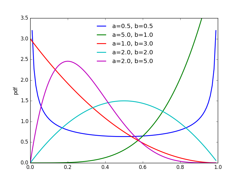
Beta分布的峰值在  a−1a+b−2  处取得，这一点在概率密度函数的曲线中可清晰地看出。

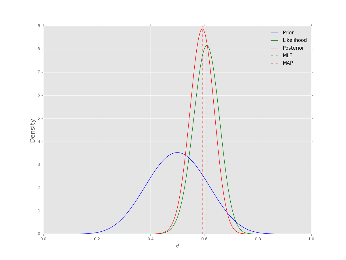
先验为  Beta  分布，似然为二项分布时的后验分布

p(θ)=θa−1(1−θ)b−1B(a,b)p(X|θ)=(nk)θk(1−θ)n−kp(θ|X)=θa+k−1(1−θ)b+n−k−1B(a+k,b+n−k)

import numpy as np
import scipy.stats as st
import matplotlib.pyplot as plt

n, k = 100, 61
p = k/n
rv = st.binom(n, p)

a, b = 10, 10
prior = st.beta(a, b)
poster = st.beta(a+k, b+n-k)

thetas = np.arange(0, 1, .001)
plt.figure(figsize=(12, 9))
plt.style.use('ggplot')
plt.plot(thetas, prior.pdf(thetas), 'b', label='Prior')
plt.plot(thetas, n*st.binom(n, thetas).pmf(k), 'g', label='Likelihood')
plt.plot(thetas, poster.pdf(thetas), 'r', label='Poster')

plt.axvline(p, c='g', ls='--', label='MLE', alpha=.4)
plt.axvline((a+k-1)/(a+b+n-2), c='r', ls='--', label='MAP', alpha=.4)
plt.legend(frameon=False)
plt.xlabel(r'$\theta$', fontsize=14)
plt.ylabel('Density', fontsize=16)
plt.show()
 
 
1
2
3
4
5
6
7
8
9
10
11
12
13
14
15
16
17
18
19
20
21
22
23
24
25
 
 
1
2
3
4
5
6
7
8
9
10
11
12
13
14
15
16
17
18
19
20
21
22
23
24
25