R1 Lecture 10 Class Notes

R1 Lecture 10 Class Notes

By YU, Xiang

May 5 2015

假设检验: 均值

Student’s t-test

One-sample t-test

理论基础

1.为了做单样本t检验,需要计算 $t$ 统计量的值：

$$t=\frac{\bar{x}-\mu_0}{s/\sqrt{n}}$$

$\bar{x}$ 是样本均值(sample mean),
$s$ 是样本标准差(sample standard deviation),
$n$ 是样本容量(sample size)

2.需要计算在给定的 $\alpha$ 下, $t-statistic$ 允许的取值范围

x <- seq(-4,4,0.1)
y <- dt(x,3)
plot(x,y,type="l")
abline(v=c(qt(0.025,3),qt(0.975,3)),col="red",lty=2)
rect(-5,-0.1,qt(0.025,3),0.4,border=FALSE,col=rgb(1,0,0,0.1))
rect(qt(0.975,3),-0.1,5,0.4,border=FALSE,col=rgb(1,0,0,0.1))
text(c(-3.7,3.7),c(0.2,0.2),"Rejection Region",srt=-90,cex=2)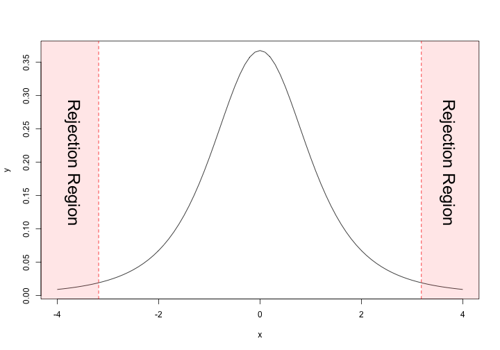

3.若 $t-statistic$ 在允许范围内,则接受原假设;否则拒绝原假设,接受备择假设

参考程序

my_t_test <- function(sample,mu,alpha=0.05){
    t_stat <- (mean(sample)-mu)/sd(sample)*sqrt(length(sample))
    q1 <- qt(alpha/2,length(sample)-1)
    q2 <- qt(1-alpha/2,length(sample)-1)
    if(t_stat > q1 & t_stat < q2){
        print("Accept the NULL Hypothesis")
    }
    else{
        print("Reject the NULL Hypothesis")
    }
}

一个检验的例子

# 使用iris数据集测试
str(iris)

## 'data.frame':    150 obs. of  5 variables:
##  $ Sepal.Length: num  5.1 4.9 4.7 4.6 5 5.4 4.6 5 4.4 4.9 ...
##  $ Sepal.Width : num  3.5 3 3.2 3.1 3.6 3.9 3.4 3.4 2.9 3.1 ...
##  $ Petal.Length: num  1.4 1.4 1.3 1.5 1.4 1.7 1.4 1.5 1.4 1.5 ...
##  $ Petal.Width : num  0.2 0.2 0.2 0.2 0.2 0.4 0.3 0.2 0.2 0.1 ...
##  $ Species     : Factor w/ 3 levels "setosa","versicolor",..: 1 1 1 1 1 1 1 1 1 1 ...

my_t_test(iris[1:50,1],5)

## [1] "Accept the NULL Hypothesis"

my_t_test(iris[1:50,1],7)

## [1] "Reject the NULL Hypothesis"

当然,普通青年会选择使用 $R\ package: stats$ 中的 $t.test$

Description:

     Performs one and two sample t-tests on vectors of data.

Usage:

     t.test(x, ...)

     ## Default S3 method:
     t.test(x, y = NULL,
            alternative = c("two.sided", "less", "greater"),
            mu = 0, paired = FALSE, var.equal = FALSE,
            conf.level = 0.95, ...)

     ## S3 method for class 'formula'
     t.test(formula, data, subset, na.action, ...)

# iris数据集中setosa和versicolor两类的Sepal.Length的均值是否相等
t.test(iris[1:50,1],iris[51:100,1])

## 
##  Welch Two Sample t-test
## 
## data:  iris[1:50, 1] and iris[51:100, 1]
## t = -10.521, df = 86.538, p-value < 2.2e-16
## alternative hypothesis: true difference in means is not equal to 0
## 95 percent confidence interval:
##  -1.1057074 -0.7542926
## sample estimates:
## mean of x mean of y 
##     5.006     5.936

# var.equal默认值为FALSE,此时使用 [Welch's t-test](http://en.wikipedia.org/wiki/Welch%27s_t_test)
# 如果已知两组数据方差相等,可修改 *var.equal=TRUE*
t.test(iris[1:50,1],iris[51:100,1],var.equal=TRUE)

## 
##  Two Sample t-test
## 
## data:  iris[1:50, 1] and iris[51:100, 1]
## t = -10.521, df = 98, p-value < 2.2e-16
## alternative hypothesis: true difference in means is not equal to 0
## 95 percent confidence interval:
##  -1.1054165 -0.7545835
## sample estimates:
## mean of x mean of y 
##     5.006     5.936

使用t-test的前提: 样本满足正态性

如何检验样本是否满足这一正态性假设?

Shapiro-Wilk Normality Test

Description:

     Performs the Shapiro-Wilk test of normality.

Usage:

     shapiro.test(x)

shapiro.test(iris[1:50,1])

## 
##  Shapiro-Wilk normality test
## 
## data:  iris[1:50, 1]
## W = 0.9777, p-value = 0.4595

shapiro.test(iris[51:100,1])

## 
##  Shapiro-Wilk normality test
## 
## data:  iris[51:100, 1]
## W = 0.9778, p-value = 0.4647

作业

写一个函数,完成两独立样本的t检验(样本容量可相等可不相等,方差相等)

my_t_test2 <- function(sample_1,sample_2,alpha=0.05){
    ...
}

可以参考以下公式:

$$t=\frac{\bar{X_{1}}-\bar{X_{2}}}{s_{X_{1}X_{2}}\centerdot\sqrt{\frac{1}{n_{1}}+\frac{1}{n_{2}}}}$$

$$s_{X_{1}X_{2}}=\sqrt{\frac{(n_{1}-1)s_{X_{1}}^{2}+(n_{2}-1)s_{X_{2}}^{2}}{n_{1}+n_{2}-2}}$$