【数据挖掘】期末

最新推荐文章于 2024-05-20 19:08:38 发布

鱼树C

最新推荐文章于 2024-05-20 19:08:38 发布

阅读量573

点赞数 12

分类专栏：数据挖掘选修文章标签：数据挖掘人工智能 python

本文链接：https://blog.csdn.net/yv_shu/article/details/128415217

版权

数据挖掘选修专栏收录该内容

5 篇文章 2 订阅

订阅专栏

前言

唉，这里是39度的羊半夜爬起来写的{{{(>_<)}}}，这次真是想吐槽一下了，老师可能确实是太高看我们了，也不知道上课讲了啥，这次让用图神经网络？据我所知图神经网络是人工智能大后期的东西了，不过抠字眼的话，好像也没说搭建图神经网络进行训练，只说了预测，另外，需要训练得到的那个矩阵好像已经给了？所以我只进行了预测，没有进行神经网络的搭建和训练。

注意

不建议跑我这个代码，可能要“非常久”，代码与dataset文件夹处于同一目录下，另外去把标准的Human_Sls.csv下载下来放到dataset文件夹中，用于与预测结果进行比较。最后就是还请不要无脑拷贝，代码无所谓，至少文字部分别。…有bug也请不要联系我，我也不关心。

数据集分析

合成致死性(SL)是发现抗癌药物靶点的一个很有希望的方法。单个基因可能对癌细胞没有致死性，而当两个基因相互作用时，可能具备致死性。

对给定数据集进行分析，可以看到有Gene_GO_similarity、gene_list、Gene_PPI_similarity、Human_Sls这么几个数据集，其中gene_list记录了实验用到的所有基因，Human_Sls记录了两个基因之间的致死性关系，但是好多基因对之间的致死性关系未知，所以需要对其进行预测，Gene_GO_similerity与Gene_PPI_similarity记录了两个基因之间的相似性，根据名称可以知道，这些关系收集自GO、PPI。
所以，可以认为这些数据已经建模完成，可以将其存储为二维数组或矩阵进行计算。
其中主要需要用到的是Human_Sls这个数据集，其中0 表示两个基因对之间的关系未知，非零表示两个基因对之间的一个致死性分数，比如可以认为大于0.5具有致死性、小于0.5不具有致死性，要注意: 未知两个基因之间的致死性关系和两个基因之间不具有致死性是两个不同的概念。
另外还可以用到Gene_GO_similarity这个数据集进行辅助，其中每个数值描述了两个基因之间的相似性，可以利用两个基因之间的相似性信息对未知致死性的基因对之间的致死性进行预测。

代码

SL描述了两个基因对之间的致死性关系，但是两个基因之间的致死性关系实际上是很多因素的影响的，这些因素可能包括细胞成分、分子功能、化合物等等，而知识图谱就是描述某些数据之间的数据库，我们可以将上述的这些影响因素使用知识图谱存储起来，通过有监督方式的学习过程，通过这些信息构建一个基因相似性关系，通过多轮的学习过程，不断更新这个基因相似性关系，之后通过相似性预测基因之间的致死性信息。
可以发现，数据集提供了基因对之间的相似性信息，所以通过有监督的方式得到基因相似性关系的过程认为已经完成了，之后需要对两个未知致病性关系的基因对之间的致病性进行预测。
大致思路如下：
在这里插入图片描述

以上图为例，左图记录了两个基因之间的相似性信息，右图记录了两个基因之间的致死性信息，可以看到，1-2、1-3、2-3、2-4之间的致死性信息是未知的，倘若我们要预测1-4之间的致死性关系：
已知的是1与其余各个基因之间的相似性，可以首先寻找与4之间的致死性关系已知的基因，比如这里的2（2-4：0.5），之后寻找1与2之间的相似性（0.1），将二者相乘得到由2结点传递给1-4的致死性关系（0.05），由于是无向图，4-1之间的致死性信息也可以用相同方式求出（0.36+0.35=0.71），可以考虑将二者相加作为1-4之间的致死性分数（0.76）。0.2+0.21+0.32
按上述策略进行一次更新之后的基因之间的致死性关系：
在这里插入图片描述

可以发现，在进行这样的一次计算之后，相当于使用已知的基因之间的致死性和基因相似性信息对未知的基因之间的相似性信息进行了一次更新，这时就会出现一个问题，仅通过上述方式进行一次更新可能导致某些基因致死性信息未被更新，因为是存在孤立的顶点的，他们不与其余顶点相连，所以可以考虑进行多次更新；另外，如果按照上述求和的方案，不难想象，随着更新次数的增加，两个基因之间的致死性关系将会持续增大，这不是我们想要的，可以考虑求平均、只用相似性最大的基因的信息进行更新等。

导入库

import numpy as np
import pandas as pd
import matplotlib.pyplot as plt  # 导入 Matplotlib 工具包
import networkx as nx  # 导入 NetworkX 工具包
from sklearn import metrics

数据预处理

# Gene_GO_similarity.txt记录了两个基因之间的相似性

f = open(r"./dataset/Gene_GO_similarity.txt")
Gene_GO_similarity = f.readlines()

gene_similarity = [[i for i in line.split(" ")] for line in Gene_GO_similarity]
i = 0
for s in range(len(gene_similarity)):
    gene_similarity[i][-1] = gene_similarity[i][-1].strip("\n")
i = i+1

gene_similarity = np.array(gene_similarity).astype(float)

# gene_list.txt记录了这次实验用的所有基因\n",

f = open(r"./dataset/gene_list.txt")
gene_list_data = f.readlines()
f.close()
i = 0
for gene in gene_list_data:
    gene_list_data[i] = gene_list_data[i].strip("\n")
i = i+1
# 创建一个字典对所有基因进行编号\n",
gene_list = dict()
i = 0
for gene in gene_list_data:
    gene_list[gene]=i
i = i+1

# human_Sls.txt中记录了已知的人类不同基因之间的致死性\n",

f = open(r"./dataset/Human_Sls.txt")
human_Sls_data = f.readlines()
f.close()
human_Sls_tmp = [[i for i in line.split("\t")]for line in human_Sls_data]
i = 0
for s in human_Sls_tmp:
    human_Sls_tmp[i][2] = s[2].strip("\n")
i = i+1

human_Sls = np.zeros((6375, 6375))
for s in human_Sls_tmp:
    human_Sls[gene_list[s[0]]][gene_list[s[1]]] = s[2]
    human_Sls[gene_list[s[1]]][gene_list[s[0]]] = s[2]
human_Sls = human_Sls.astype(float)

# human_Sls.csv中记录了已知的目前所有人类基因之间的致死性情况\n",

f = pd.read_csv(r"./dataset/Human_SL.csv")

human_Sls_test = np.zeros((6375, 6375))
for i in range(f.shape[0]):
    if f.iloc[i,0] in gene_list.keys() and f.iloc[i,1] in gene_list.keys():
        human_Sls_test[gene_list[f.iloc[i,0]]][gene_list[f.iloc[i,1]]] = f.iloc[i,2]
        human_Sls_test[gene_list[f.iloc[i,1]]][gene_list[f.iloc[i,0]]] = f.iloc[i,2]

至此，数据预处理完成:
Gene_similarity: 二维数组，存储了两个基因之间的相似性
gene_list: 字典类型，以各个基因名为键标识各个基因编号
human_Sls: 二维数组，存储实验过程中已知的各个基因之间的致死性信息
human_Sls_test: 二维数组，从官网下载的标准的各个基因之间的致死性信息

预测未知基因之间的致死性关系

已知: 部分基因之间的致死性信息、某两个基因之间的相似性
目标: 预测其余未知致死性信息的基因之间的致死性
思路: 由于已知两个基因之间的相似性，所以我们可以认为“相似的基因之间的致死性信息也相似”
对于未知致死性关系的基因，在图中寻找与其相似的基因，接着寻找该基因目标基因的致死性关系

train_Set = np.array([[i for i in j]for j in human_Sls]).astype(float)
tmp_Set =  np.array([[i for i in j]for j in human_Sls]).astype(float)

首先利用已知致死性关系的基因和相似性对未知致死性关系的基因进行一次更新
更新方式:
如果基因A与基因B的致死性关系未知，寻找所有与A相似的基因C，若C与B之间的致死性关系已知，则将A与C的相似性* C与B的致死性
之后寻找所有与B相似的基因D，若D与A之间的致死性关系已知，则将B与D的相似性* D与A的致死性
最后将上述两个计算值相加对未知的致死性进行一次更新

for r in range(human_Sls.shape[0]):
    print(r)
    c = r
    while c<human_Sls.shape[1]:
        if human_Sls[r][c]==0:
            tmp_Set[r][c] = tmp_Set[c][r] = np.dot(gene_similarity[r], human_Sls[:,c])+np.dot(gene_similarity[c], human_Sls[:,r])
        else:
            tmp_Set[r][c] = tmp_Set[c][r] = human_Sls[r][c]
        c = c+1

只通过上述方式得到的结果与标准致死性之间有很大的差距，这里考虑对每个基因再次进行信息更新，如果仍按上述方式进行更新，可以想到，随着信息的不断增加，两个基因之间的致死性将会持续增大，这不是我们想要的。
这里考虑使用相似基因与目标基因的致死性之和的平均值进行更新。

train_Set = np.array([[i for i in j]for j in tmp_Set]).astype(float)
for r in range(human_Sls.shape[0]):
    # print(r)
    c = r
    while c<human_Sls.shape[1]:
        if human_Sls[r][c]==0:
            tmp_Set[r][c] = tmp_Set[c][r] = 10*(np.dot(gene_similarity[r], train_Set[:,c])/np.count_nonzero(train_Set[:,c])
            +np.dot(gene_similarity[c], human_Sls[:,r])/np.count_nonzero(train_Set[:,r]))
        else:
            tmp_Set[r][c] = tmp_Set[c][r] = human_Sls[r][c]
        c = c+1
# print(tmp_Set[r][0])

经过过上述方式得到的结果与标准致死性之间仍有很大的差距，这里考虑对每个基因再次进行信息更新，这里考虑使用相似性最大的基因与目标基因的致死性进行更新。

train_Set = np.array([[i for i in j]for j in tmp_Set]).astype(float)

for r in range(human_Sls.shape[0]):
    # print(r)
    c = r
    while c<human_Sls.shape[1]:
        if human_Sls[r][c]==0:
            tmp_Set[r][c] = tmp_Set[c][r] = np.max(gene_similarity[r])*\
            train_Set[r,np.where(gene_similarity[r] == np.max(gene_similarity[r]))[0][0]] + \
            np.max(gene_similarity[c])* \
            train_Set[r,np.where(gene_similarity[c] == np.max(gene_similarity[c]))[0][0]] 
        else:
            tmp_Set[r][c] = tmp_Set[c][r] = human_Sls[r][c]
        c = c+1
# print(tmp_Set[r][0])

至此，tmp_Set中存储最新的致死性关系信息。

图的可视化

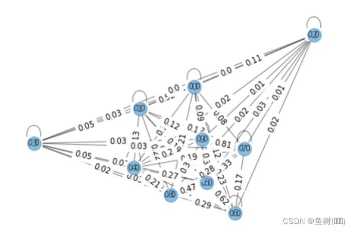
基因之间的相似性关系(只查看前10个)

simi_list = []
for r in range(10):
    c = r
    while c<10:
        simi_list.append((r,c,gene_similarity[r][c]))
        c = c+1

G = nx.Graph()  # 创建无向图
G.add_weighted_edges_from(simi_list)  # 向图中添加多条赋权边

pos = nx.spring_layout(G)
nx.draw(G, pos, with_labels=True, alpha=0.5)
labels = nx.get_edge_attributes(G, 'weight')
nx.draw_networkx_edge_labels(G, pos, edge_labels=labels)
plt.show()

在这里插入图片描述
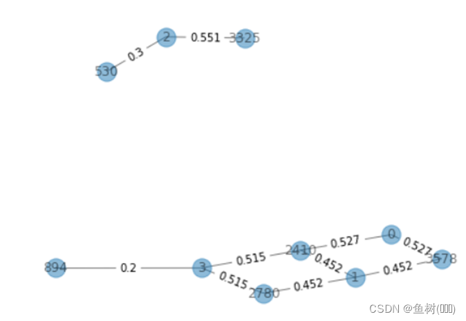
标准的致死性关系(只查看前10个)

edge_list = []
for r in range(human_Sls_test.shape[0]):
    c = r
    while c<human_Sls_test.shape[1]:
        if human_Sls_test[r][c]!=0:
            edge_list.append((r,c,human_Sls_test[r][c]))
        c = c+1

G1 = nx.Graph()  # 创建无向图
G1.add_weighted_edges_from(edge_list[:10])  # 向图中添加多条赋权边

pos = nx.spring_layout(G1)
nx.draw(G1, pos, with_labels=True, alpha=0.5)
labels = nx.get_edge_attributes(G1, 'weight')
nx.draw_networkx_edge_labels(G1, pos, edge_labels=labels)
plt.show()

在这里插入图片描述
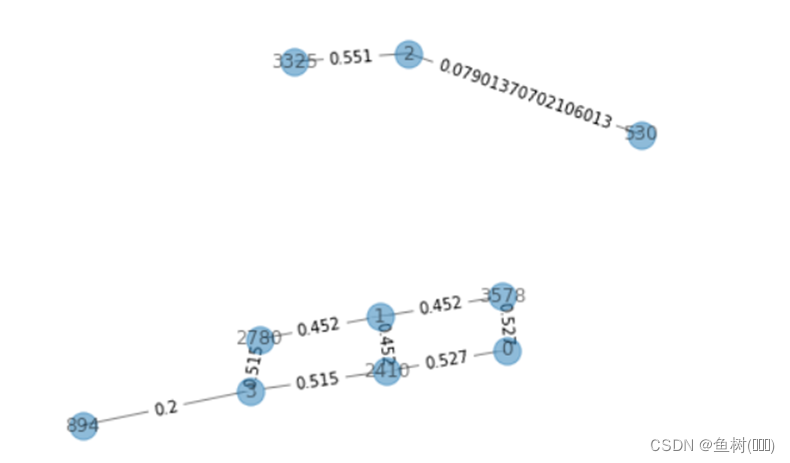
预测得到的致死性关系(只查看前10个)

edge_list2 = []
for r in range(human_Sls_test.shape[0]):
    c = r
    while c<human_Sls_test.shape[1]:
        if human_Sls_test[r][c]!=0:
            edge_list2.append((r,c,tmp_Set[r][c]))
        c = c+1

G2 = nx.Graph()  # 创建无向图
G2.add_weighted_edges_from(edge_list2[:10])  # 向图中添加多条赋权边

pos = nx.spring_layout(G2)
nx.draw(G1, pos, with_labels=True, alpha=0.5)
labels = nx.get_edge_attributes(G2, 'weight')
nx.draw_networkx_edge_labels(G2, pos, edge_labels=labels)
plt.show()

在这里插入图片描述

查看不同指标下的预测结果

label = []
pre = []
pre_label = []
i = 0
for r in range(human_Sls.shape[0]):
    for c in range(human_Sls.shape[1]):
        if human_Sls[r][c]==0 and human_Sls_test[r][c]!=0:
            if human_Sls_test[r][c]>0.5:
                label.append(1)
            else:
                label.append(0)
            if tmp_Set[r][c]>0.5:
                pre_label.append(1)
            else:
                pre_label.append(0)
            pre.append(tmp_Set[r][c])
            # print(label[i])
            # print(pre[i])
            # print("---------")
            i = i+1

fpr1, tpr1, thresholds = metrics.roc_curve(label, pre)
roc_auc1 = metrics.auc(fpr1, tpr1)  # the value of roc_auc1
print(roc_auc1)

在这里插入图片描述

precision1, recall1, _ = metrics.precision_recall_curve(label, pre)
aupr1 = metrics.auc(recall1, precision1)  # the value of roc_auc1
print(aupr1)

在这里插入图片描述

f1 = metrics.f1_score(pre_label, label)
print(f1)

在这里插入图片描述

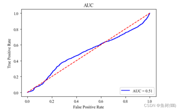
绘制AUC曲线

plt.rc('font', family='Times New Roman')

plt.plot(fpr1, tpr1, 'b', label='AUC = %0.2f' % roc_auc1)
plt.legend(loc='lower right')
plt.plot([0, 1], [0, 1], 'r--')
# plt.xlim([0, 1])  # the range of x-axis
# plt.ylim([0, 1])  # the range of y-axis
plt.xlabel('False Positive Rate')  # the name of x-axis
plt.ylabel('True Positive Rate')  # the name of y-axis
plt.title('AUC')  # the title of figure
plt.show()

在这里插入图片描述

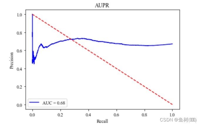
绘制AUPR曲线

plt.rc('font', family='Times New Roman')

plt.plot(recall1, precision1, 'b', label='AUC = %0.2f' % aupr1)
plt.legend(loc='lower left')
plt.plot([1, 0], 'r--')
# plt.xlim([0, 1])  # the range of x-axis
# plt.ylim([0, 1])  # the range of y-axis
plt.xlabel('Recall')  # the name of x-axis
plt.ylabel('Precision')  # the name of y-axis
plt.title('AUPR')  # the title of figure
plt.show()

在这里插入图片描述

实验总结

呃，头疼≡(▔﹏▔)≡

鱼树C

关注

12
点赞
踩
3

收藏

觉得还不错? 一键收藏
打赏
0
评论
【数据挖掘】期末

SL描述了两个基因对之间的致死性关系，但是两个基因之间的致死性关系实际上是很多因素的影响的，这些因素可能包括细胞成分、分子功能、化合物等等，而知识图谱就是描述某些数据之间的数据库，我们可以将上述的这些影响因素使用知识图谱存储起来，通过有监督方式的学习过程，通过这些信息构建一个基因相似性关系，通过多轮的学习过程，不断更新这个基因相似性关系，之后通过相似性预测基因之间的致死性信息。
复制链接

扫一扫