对抗生成网络学习（十四）——DRAGAN对模型倒塌问题的处理和生成图像质量评价(tensorflow实现)

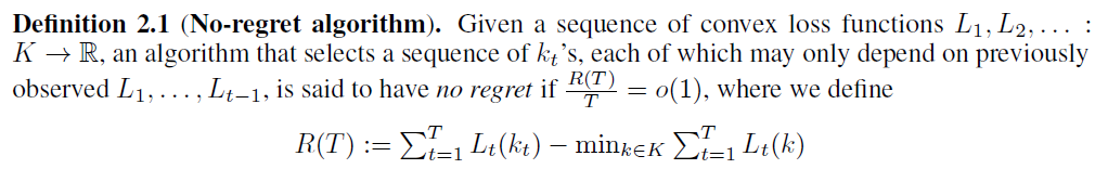
一、背景

之前在做GAN主要是关注GAN的应用，找了一些比较好的例子实现了下，后面还会持续做这方面的工作。今天来看看DRAGAN对于GAN中一些问题的处理方法，也为今后这方面的研究做一部分基础工作吧，我们不仅应该了解GAN能做什么，还应该了解GAN的问题及解决方法。

DRAGAN是Naveen Kodali等人于2017年5月发表的一篇文章《ON CONVERGENCE AND STABILITY OF GANS》，虽然文章发表的比较早，不过这篇文章的思路还是非常值得我们去学习，这篇文章的重点我会放在一些分析上，后面的实验过程我暂时先用MNIST数据集做实验，重点会分析一部分代码，总之先对文章进行一个详细的解读吧。

[1]文章链接：https://arxiv.org/pdf/1705.07215.pdf

二、DRAGAN原理

很遗憾的是，网上几乎没有对这篇文章的解读，所以我就根据自己的理解来解读一下这篇文章的工作。

我先把文章的摘要部分截取出来：

We propose studying GAN training dynamics as regret minimization, which is in contrast to the popular view that there is consistent minimization of a divergence between real and generated distributions. We analyze the convergence of GAN training from this new point of view to understand why mode collapse happens. We hypothesize the existence of undesirable local equilibria in this non-convex game to be responsible for mode collapse. We observe that these local equilibria often exhibit sharp gradients of the discriminator function around some real data points. We demonstrate that these degenerate local equilibria can be avoided with a gradient penalty scheme called DRAGAN. We show that DRAGAN enables faster training, achieves improved stability with fewer mode collapses, and leads to generator networks with better modeling performance across a variety of architectures and objective functions.

简而言之，作者提出一个观点，GAN的训练过程是作为一种regret minimization（后悔最小化？不太明白专业翻译是啥）而非出传统观点所认为的consistent minimization（持续最小化）。猜测模型倒塌（mode collapse）是由于在非凸情况下出现了局部平衡，作者观测到局部平衡总是在判别函数中的真实数据周围表现出了尖锐的梯度，因此作者提出DRAGAN，在模型中引入梯度惩罚机制以避免局部平衡。结果表明，DRAGAN能够更快训练，且更稳定，很少出现模型倒塌（mode collapse）现象。

我们知道，GAN是能够学习数据分布的，模型驱动一般是用梯度下降，但是，GAN是不稳定的，GAN会一定程度上引起模型倒塌（mode collapse）现象。传统观点认为引起该现象的原因是由于训练过程中尝试极小化强发散（minimize a strong divergence）。

作者指出，GAN的训练是一种博弈，生成器和判别器都是用的无悔算法（no-regret algorithms）。然而，这种方式会导致，非凸（non-convex）情况（常常用于深度神经网络）下，收敛的不稳定（convergence results do not hold）。在非凸博弈中，通常来看，全局有悔极小化（global regret minimization）和平衡计算（equilibrium computation）是非常困难的。并且，梯度下降法最终还会陷入循环或者在一些情况下收敛于局部平衡。作者猜测上面的两点问题分别导致了陷入循环和模型倒塌，然而，对于陷入循环现象无法探测，因此作者重点关注模型倒塌的问题。

还是回到前面的问题，模型倒塌是由于判别器中出现了过于尖锐的梯度，为了解决这个问题，可以加入单隐含层的神经网络，这也解释了为什么WGAN能够减轻模型倒塌的现象（可参考：对抗神经网络学习（四）——WGAN+爬虫生成皮卡丘图像(tensorflow实现)），因此作者加入了梯度惩罚机制，提出DRAGAN（Deep Regret Analytic Generative Adversarial Networks），作者的主要贡献可以总结为以下几点：

• We propose a new way of reasoning about the GAN training dynamics - by viewing AGD as regret minimization. （提出了一个GAN训练过程中出现问题的一种新的原因——将梯度下降作为regret minimization）
• We provide a novel proof for the asymptotic convergence of GAN training in the nonparametric limit and it does not require the discriminator to be optimal at each step.（对于GAN在非参限制下的渐进收敛提出了一种新的证明）
• We discuss how AGD can converge to a potentially bad local equilibrium in non-convex games and hypothesize this to be responsible for mode collapse during GAN training.（讨论了梯度下降在非凸博弈中如何收敛到局部平衡）
• We characterize mode collapse situations with sharp gradients of the discriminator function around some real data points.（判别函数周围的真实数据点所产生的尖锐梯度会导致模型倒塌）
• A novel gradient penalty scheme called DRAGAN is introduced based on this observation and we demonstrate that it mitigates the mode collapse issue.（一种新的梯度惩罚项，建立DRAGAN）

前面主要是作者对文章内容的综述，下面是部分相关背景工作：（这里实在是懒得打公式了，就先截图了）

为了做进一步实验，首先我们需要先了解GAN中的一些内容，对于GAN来说，生成器和判别器的cost function可以定义为：

对于整个模型来说，也就是：

对于凸凹情况来讲，若要满足下面的方程：

此时，可以认为生成器和判别器的博弈达到了一个平衡状态。观测这种平衡最好的方法则是regret minimization，为了解释这个方法，需要先介绍无悔算法（no-regret algorithms）：

假定我们给出凸损失函数序列L1,L2, . . . :K ——> R，我们选出前t个序列记为Kt，无悔算法即指的是：

这里我们就可以用无悔算法找到GAN博弈的结果J(·,·)。推导过程如下，若经过t轮博弈，生成器的损失函数可以表示为，判别器的损失函数可以表示为，T轮博弈之后：

换句话说：

下面是关于模型倒塌现象出现的解决办法：

模型倒塌的原因前面也介绍过了，这种尖锐的梯度，会使得多个z矢量映射到单个输出x，造成博弈的退化平衡（实际表现出来也就是输入的多组变量都会产生一致的结果），为了减少这种现象，可以对判别器添加惩罚项：

这个方法也确实能够提高模型训练的稳定性。这也解释了为什么WGAN能一定程度上解决模型倒塌，进一步的研究，这种机制非常难达到，一旦过度惩罚（over-penalized），判别器则会引入一些噪声，因此更好的惩罚项应该如下设置：

最后，出于一些经验性的优化考虑，作者最终所采用的惩罚项为：

左图是训练次数与inception score（该参数用来评价GAN生成图像质量的好坏，不过有一定缺陷）的关系图，右边是相应的判别器的梯度均方值，可以看到，图像中出现了变化剧烈的地方，这也就是产生模型倒塌的原因。

另外的一些细节包括：

• We use the vanilla GAN objective in our experiments, but our penalty improves stability using other objective functions as well. This is demonstrated in section 3.3. （实验使用了vanilla GAN对象，但是惩罚项是用了其他对象）
• The penalty scheme used in our experiments is the one shown in equation 1. （惩罚机制使用的是上文提到的）
• We use small pixel-level noise but it is possible to find better ways of imposing this penalty. However, this exploration is beyond the scope of our paper.（对于该惩罚项中的噪声采用的是小的像素级噪声，但其实还有更好的方法）
• The optimal configuration of the hyperparameters for DRAGAN depends on the architecture, dataset and data domain. We set them to be λ ~ 10, k = 1 and c ~ 10 in most of our experiments.（超参数的优化与模型结构，数据集，数据域有关。）

下面作者展示了一下加入梯度惩罚项后的变化，变化前的IS得分（一种评价生成图像质量的因子）变化：

变化后的得分：

明显可以看到图像中明显减少剧烈变化的地方，这也就是说一定程度上减轻了模型倒塌。

最后作者提到，现有模型中，有很多采用正则化来限制判别器梯度的方法，思路与作者的很类似，比较典型的是LS-GAN和WGAN-GP；在LS-GAN中，模型在判别器中引入Lipschitz constraint，并做了如下约束：

相似的是，WGAN-GP也是对判别器进行约束：

这两种思路非常相似，作者将其称之为“coupled penalties”（双重惩罚？）。

而WGAN-GP仍然没有对任意成对的真假图像进行处理（这里应该指的是没有加入偏执项），根据现有文献，在成对的真假图像中，理想判别器是有着1范数梯度（norm-1 gradients）的，且这些成对样本的联合分布为泊松分布（π）。而这也是DRAGAN和其他方法的不同之处，作者将自己的方法称之为“local penalties”（局部惩罚）。当然，作者也指出了coupled penalties存在的问题：

• With adversarial training finding applications beyond fitting implicit generative models, penalties which depend on generated samples can be prohibitive. （惩罚项可能会被抑制）
• The resulting class of functions when coupled penalties are used will be highly restricted compared to our method and this affects modeling performance. We refer the reader to Figure 4 and appendix section 5.2.2 to see this effect.（coupled penalties会使结果被严重限制）
• Our algorithm works with AGD, while WGAN-GP needs multiple inner iterations to optimize D. This is because the generated samples can be anywhere in the data space and they change from one iteration to the next. In contrast, we consistently regularize D(x) only along the real data manifold.（作者的算法可以直接使用自适应梯度下降，但是WGAN-GP则需要内部多次迭代来优化判别器）

最后是作者的一些小实验，这里就不多说了，贴出一个关于Swissroll数据（瑞士卷）的实验吧：

图中橙色的是真实数据，绿色的是生成的样本，背景中类似等高线的是水平集（一种region-based图像分割方法），从上到下的依次是普通的GAN，WGAN-GP，DRAGAN，从左到右依次是训练的不同阶段，通过这些图也能够比较明显的看出来，DRAGAN能够很好的拟合真实数据。

实验的代码主要参考：

[2]https://github.com/hwalsuklee/tensorflow-generative-model-collections

不过自己在运行的过程中，发现原有代码的保存图像还有运行程序当中，有一点小问题，因此做了一定改进。

三、DRAGAN实现

1. 文件结构

DRAGAN所需要的文件结构包括：

-- utils.py                          # 辅助文件
-- ops.py                            # 图层文件
-- dragan.py                         # 主文件
-- mnist_data                        ###### 需要自己准备数据集
    |------ 0
            |------ image1.jpg
            |------ image2.jpg
            |------ ......
    |------ 1
            |------ image1.jpg
            |------ image2.jpg
            |------ ......
    |------ 2
    |------ ......
    |------ 9
            |------ image1.jpg
            |------ image2.jpg
            |------ ......
          

和传统mnist数据集不同的是，这次我是将mnist数据集的图片做好，按类别放在了不同文件夹里，这样也一定程度上可以将该方法用于其他数据。至于如何制作数据集，这里就不再多说了，可以参考：对抗神经网络学习（一）——GAN实现mnist手写数字生成(tensorflow实现)。当然了，实际上DRAGAN是非监督模型，不需要这些标签也仍然可以顺利运行。

2. 辅助文件utils.py

utils.py文件主要定义了一些保存图像，加载变量的操作，我对原代码中的很多功能进行了删除，只保留了两个函数，下面摘一些比较关键的代码：

首先是保留关键变量：

def show_all_variables():
    import tensorflow as tf
    import tensorflow.contrib.slim as slim
    model_vars = tf.trainable_variables()
    slim.model_analyzer.analyze_vars(model_vars, print_info=True)

其次我们需要对实验生成的结果进行绘制，这里将64张图贴到一起，这段代码是参考了之前写GAN时的代码，觉得更简单好用，函数如下：

def show_result(batch_res, fname, grid_size=(8, 8), grid_pad=0, image_height=28, image_width=28):
    from skimage import io
    import numpy as np
    batch_res = 0.5 * batch_res.reshape((batch_res.shape[0], image_height, image_width)) + 0.5
    # 重构显示图像格网的参数
    img_h, img_w = batch_res.shape[1], batch_res.shape[2]
    grid_h = img_h * grid_size[0] + grid_pad * (grid_size[0] - 1)
    grid_w = img_w * grid_size[1] + grid_pad * (grid_size[1] - 1)
    img_grid = np.zeros((grid_h, grid_w), dtype=np.uint8)
    for i, res in enumerate(batch_res):
        if i >= grid_size[0] * grid_size[1]:
            break
        img = res * 255.
        img = img.astype(np.uint8)
        row = (i // grid_size[0]) * (img_h + grid_pad)
        col = (i % grid_size[1]) * (img_w + grid_pad)
        img_grid[row:row + img_h, col:col + img_w] = img
    io.imsave(fname, img_grid)

3. 图层文件ops.py

ops.py文件中定义了很多图层相关的操作。下面来一一说明。

首先是BN（batch normalization）层，主要功能就是进行归一化，一定程度上减少过拟合：

import tensorflow as tf

def bn(x, is_training, scope):
    return tf.contrib.layers.batch_norm(x,
                                        decay=0.9,
                                        updates_collections=None,
                                        epsilon=1e-5,
                                        scale=True,
                                        is_training=is_training,
                                        scope=scope)

接下来是一对常用的卷积和反卷积操作，这两个操作有现成的API，只不过将它们封装成函数会更方便一些：

def conv2d(input_, output_dim, k_h=5, k_w=5, d_h=2, d_w=2, stddev=0.02, name="conv2d"):
    with tf.variable_scope(name):
        w = tf.get_variable('w', [k_h, k_w, input_.get_shape()[-1], output_dim],
              initializer=tf.truncated_normal_initializer(stddev=stddev))
        conv = tf.nn.conv2d(input_, w, strides=[1, d_h, d_w, 1], padding='SAME')

        biases = tf.get_variable('biases', [output_dim], initializer=tf.constant_initializer(0.0))
        conv = tf.reshape(tf.nn.bias_add(conv, biases), conv.get_shape())

        return conv

def deconv2d(input_, output_shape, k_h=5, k_w=5, d_h=2, d_w=2, name="deconv2d", stddev=0.02, with_w=False):
    with tf.variable_scope(name):
        # filter : [height, width, output_channels, in_channels]
        w = tf.get_variable('w', [k_h, k_w, output_shape[-1], input_.get_shape()[-1]],
                            initializer=tf.random_normal_initializer(stddev=stddev))

        deconv = tf.nn.conv2d_transpose(input_, w, output_shape=output_shape, strides=[1, d_h, d_w, 1])

        biases = tf.get_variable('biases', [output_shape[-1]], initializer=tf.constant_initializer(0.0))
        deconv = tf.reshape(tf.nn.bias_add(deconv, biases), deconv.get_shape())

        if with_w:
            return deconv, w, biases
        else:
            return deconv

最后就是leakyRelu和线性函数，这里也直接给出：

def lrelu(x, leak=0.2, name="lrelu"):
    return tf.maximum(x, leak*x)

def linear(input_, output_size, scope=None, stddev=0.02, bias_start=0.0, with_w=False):
    shape = input_.get_shape().as_list()

    with tf.variable_scope(scope or "Linear"):
        matrix = tf.get_variable("Matrix", [shape[1], output_size], tf.float32,
                 tf.random_normal_initializer(stddev=stddev))
        bias = tf.get_variable("bias", [output_size],
        initializer=tf.constant_initializer(bias_start))
        if with_w:
            return tf.matmul(input_, matrix) + bias, matrix, bias
        else:
            return tf.matmul(input_, matrix) + bias

4. 模型文件dragan.py

dragan.py文件的内容比较多，包括读取数据，定义dragan的相关操作，主函数控制流程等，下面来简要进行说明。

首先我们需要导入相关的库和定义关键的超参数（当然这些参数你也可以封装到主函数里）：

import os, glob
from skimage import io, transform
import time

from ops import *
from utils import *

epochs = 1000
batch_size = 64
z_dim = 128
checkpoint_dir = './DRAGAN/checkpoint/'
result_dir = './DRAGAN/result/'
dataset_dir = 'mnist_data/'

接下来是读取数据部分，这里我的思路是，读取文件夹下的所有数据，按子文件夹的编号为其制作标签，同时考虑是否将标签制作成onehot编码格式，最后将数据集的80%用作训练，20%用作测试，这部分的代码为：

def get_data(data_path, onehot=False, train_data_rate=0.8, image_height=28, image_width=28):

    def label_to_onehot(labels):
        n_sample = len(labels)
        n_class = max(labels) + 1
        onehot_labels = np.zeros((n_sample, n_class))
        onehot_labels[np.arange(n_sample), labels] = 1
        return onehot_labels

    # 找到路径下的所有子文件夹
    cate = [data_path + f for f in os.listdir(data_path) if os.path.isdir(data_path + f)]
    # 设置两个变量用来存放图像和标签
    imgs = []
    labels = []
    # 循环读取每张图片并制作标签
    for idx, folder in enumerate(cate):
        for im in glob.glob(folder + '/*.jpg'):
            print('reading the images:%s' % im)
            img = io.imread(im)
            img = (img < 127) * (255 - img)
            img = transform.resize(img, (image_height, image_width))
            # img = tf.image.per_image_standardization(img)
            imgs.append(img)
            labels.append(idx)

    if onehot:
        labels = label_to_onehot(labels)

    # 随机打乱数据
    image_num = np.asarray(imgs, np.float32).shape[0]
    arr = np.arange(image_num)
    np.random.shuffle(arr)
    data = np.asarray(imgs, np.float32)[arr]
    label = np.asarray(labels, np.int32)[arr]

    # 将所有数据分为训练集和验证集
    s = np.int(image_num * train_data_rate)
    x_train = data[:s].reshape(-1, image_height, image_width, 1)
    y_train = label[:s]
    x_val = data[s:].reshape(-1, image_height, image_width, 1)
    y_val = label[s:]

    return x_train, y_train, x_val, y_val, image_num

接下来才是最最关键的部分，也就是draGAN模型的构建，draGAN主要是在infoGAN的基础上进行的，这里我主要参考原代码，做了少量改进，下面给出所有相关代码：

class DRAGAN(object):
    model_name = "DRAGAN"     # name for checkpoint

    def __init__(self, sess, epoch, batch_size, z_dim, checkpoint_dir, result_dir,dataset_dir):
        self.sess = sess
        self.dataset_dir = dataset_dir
        self.checkpoint_dir = checkpoint_dir
        self.result_dir = result_dir
        self.epoch = epoch
        self.batch_size = batch_size

        self.image_height = 28
        self.image_width = 28
        self.image_channel = 1
        self.z_dim = z_dim

        # DRAGAN parameter
        self.lambd = 0.25       # The higher value, the more stable, but the slower convergence

        # summary writer
        self.writer = tf.summary.FileWriter('./logs/' + self.model_name, self.sess.graph)

        # train
        self.learning_rate = 0.0002
        self.beta1 = 0.5

        # test
        self.sample_num = 64  # number of generated images to be saved

        # load data
        self.train_x, self.train_y, self.val_y, self.val_y, self.image_num = get_data(self.dataset_dir)
        self.num_batches = self.image_num // self.batch_size

    def discriminator(self, x, is_training=True, reuse=False):
        # Network Architecture is exactly same as in infoGAN (https://arxiv.org/abs/1606.03657)
        # Architecture : (64)4c2s-(128)4c2s_BL-FC1024_BL-FC1_S
        with tf.variable_scope("discriminator", reuse=reuse):

            net = lrelu(conv2d(x, 64, 4, 4, 2, 2, name='d_conv1'))
            net = lrelu(bn(conv2d(net, 128, 4, 4, 2, 2, name='d_conv2'), is_training=is_training, scope='d_bn2'))
            net = tf.reshape(net, [self.batch_size, -1])
            net = lrelu(bn(linear(net, 1024, scope='d_fc3'), is_training=is_training, scope='d_bn3'))
            out_logit = linear(net, 1, scope='d_fc4')
            out = tf.nn.sigmoid(out_logit)

            return out, out_logit, net

    def generator(self, z, is_training=True, reuse=False):
        # Network Architecture is exactly same as in infoGAN (https://arxiv.org/abs/1606.03657)
        # Architecture : FC1024_BR-FC7x7x128_BR-(64)4dc2s_BR-(1)4dc2s_S
        with tf.variable_scope("generator", reuse=reuse):
            net = tf.nn.relu(bn(linear(z, 1024, scope='g_fc1'), is_training=is_training, scope='g_bn1'))
            net = tf.nn.relu(bn(linear(net, 128 * 7 * 7, scope='g_fc2'), is_training=is_training, scope='g_bn2'))
            net = tf.reshape(net, [self.batch_size, 7, 7, 128])
            net = tf.nn.relu(
                bn(deconv2d(net, [self.batch_size, 14, 14, 64], 4, 4, 2, 2, name='g_dc3'), is_training=is_training,
                   scope='g_bn3'))

            out = tf.nn.sigmoid(deconv2d(net, [self.batch_size, 28, 28, 1], 4, 4, 2, 2, name='g_dc4'))

            return out

    def get_perturbed_batch(self, minibatch):
        return minibatch + 0.5 * minibatch.std() * np.random.random(minibatch.shape)

    def build_model(self):
        # some parameters
        image_dims = [self.image_height, self.image_width, self.image_channel]
        bs = self.batch_size

        """ Graph Input """
        self.inputs = tf.placeholder(tf.float32, [bs] + image_dims, name='real_images')
        self.inputs_p = tf.placeholder(tf.float32, [bs] + image_dims, name='real_perturbed_images')

        # noises
        self.z = tf.placeholder(tf.float32, [bs, self.z_dim], name='z')

        """ Loss Function """

        # output of D for real images
        D_real, D_real_logits, _ = self.discriminator(self.inputs, is_training=True, reuse=False)

        # output of D for fake images
        G = self.generator(self.z, is_training=True, reuse=False)
        D_fake, D_fake_logits, _ = self.discriminator(G, is_training=True, reuse=True)

        # get loss for discriminator
        d_loss_real = tf.reduce_mean(
            tf.nn.sigmoid_cross_entropy_with_logits(logits=D_real_logits, labels=tf.ones_like(D_real)))
        d_loss_fake = tf.reduce_mean(
            tf.nn.sigmoid_cross_entropy_with_logits(logits=D_fake_logits, labels=tf.zeros_like(D_fake)))

        self.d_loss = d_loss_real + d_loss_fake

        # get loss for generator
        self.g_loss = tf.reduce_mean(
            tf.nn.sigmoid_cross_entropy_with_logits(logits=D_fake_logits, labels=tf.ones_like(D_fake)))

        """ DRAGAN Loss (Gradient penalty) """
        # This is borrowed from https://github.com/kodalinaveen3/DRAGAN/blob/master/DRAGAN.ipynb
        alpha = tf.random_uniform(shape=self.inputs.get_shape(), minval=0.,maxval=1.)
        differences = self.inputs_p - self.inputs  # This is different from WGAN-GP
        interpolates = self.inputs + (alpha * differences)
        _, D_inter, _=self.discriminator(interpolates, is_training=True, reuse=True)
        gradients = tf.gradients(D_inter, [interpolates])[0]
        slopes = tf.sqrt(tf.reduce_sum(tf.square(gradients), reduction_indices=[1]))
        gradient_penalty = tf.reduce_mean((slopes - 1.) ** 2)
        self.d_loss += self.lambd * gradient_penalty

        """ Training """
        # divide trainable variables into a group for D and a group for G
        t_vars = tf.trainable_variables()
        d_vars = [var for var in t_vars if 'd_' in var.name]
        g_vars = [var for var in t_vars if 'g_' in var.name]

        # optimizers
        with tf.control_dependencies(tf.get_collection(tf.GraphKeys.UPDATE_OPS)):
            self.d_optim = tf.train.AdamOptimizer(self.learning_rate*5, beta1=self.beta1) \
                      .minimize(self.d_loss, var_list=d_vars)
            self.g_optim = tf.train.AdamOptimizer(self.learning_rate*5, beta1=self.beta1) \
                      .minimize(self.g_loss, var_list=g_vars)

        """" Testing """
        # for test
        self.fake_images = self.generator(self.z, is_training=False, reuse=True)

        """ Summary """
        d_loss_real_sum = tf.summary.scalar("d_loss_real", d_loss_real)
        d_loss_fake_sum = tf.summary.scalar("d_loss_fake", d_loss_fake)
        d_loss_sum = tf.summary.scalar("d_loss", self.d_loss)
        g_loss_sum = tf.summary.scalar("g_loss", self.g_loss)

        # final summary operations
        self.g_sum = tf.summary.merge([d_loss_fake_sum, g_loss_sum])
        self.d_sum = tf.summary.merge([d_loss_real_sum, d_loss_sum])

    def train(self):

        # initialize all variables
        self.sess.run(tf.global_variables_initializer())

        # graph inputs for visualize training results
        self.sample_z = np.random.uniform(-1, 1, size=(self.batch_size , self.z_dim))

        # saver to save model
        self.saver = tf.train.Saver()

        # restore check-point if it exits
        could_load, checkpoint_counter = self.load(self.checkpoint_dir)
        if could_load:
            start_epoch = int(checkpoint_counter / self.num_batches)
            start_batch_id = checkpoint_counter - start_epoch * self.num_batches
            counter = checkpoint_counter
            print(" [*] Load SUCCESS")
        else:
            start_epoch = 0
            start_batch_id = 0
            counter = 1
            print(" [!] Load failed...")

        # loop for epoch
        start_time = time.time()
        for epoch in range(start_epoch, self.epoch):

            # get batch data
            for idx in range(start_batch_id, self.num_batches):
                batch_images = self.train_x[idx*self.batch_size:(idx+1)*self.batch_size]
                if batch_images.shape[0] != self.batch_size:
                    continue
                batch_images_p = self.get_perturbed_batch(batch_images)
                batch_z = np.random.uniform(-1, 1, [self.batch_size, self.z_dim]).astype(np.float32)

                # update D network
                _, summary_str, d_loss = self.sess.run([self.d_optim, self.d_sum, self.d_loss],
                                               feed_dict={self.inputs: batch_images,
                                                          self.inputs_p: batch_images_p,
                                                          self.z: batch_z})
                self.writer.add_summary(summary_str, counter)

                # update G network
                _, summary_str, g_loss = self.sess.run([self.g_optim, self.g_sum, self.g_loss],
                                                       feed_dict={self.z: batch_z})
                self.writer.add_summary(summary_str, counter)

                # display training status
                counter += 1
                print("Epoch: [%2d] [%4d/%4d] time: %4.4f, d_loss: %.8f, g_loss: %.8f" \
                      % (epoch, idx, self.num_batches, time.time() - start_time, d_loss, g_loss))

                # save training results for every 10 steps
                if np.mod(counter, 10) == 0:
                    samples = self.sess.run(self.fake_images,
                                            feed_dict={self.z: self.sample_z})
                    show_result(samples, os.path.join(result_dir, '_train_{:02d}_{:04d}.png'.format(epoch, idx)))

            # After an epoch, start_batch_id is set to zero
            # non-zero value is only for the first epoch after loading pre-trained model
            start_batch_id = 0

            # show temporal results
            self.visualize_results(epoch)

        # save model for final step
        self.save(self.checkpoint_dir, counter)

    def visualize_results(self, epoch):
        """ random condition, random noise """

        z_sample = np.random.uniform(-1, 1, size=(self.batch_size, self.z_dim))

        samples = self.sess.run(self.fake_images, feed_dict={self.z: z_sample})
        show_result(samples, os.path.join(result_dir, '_epoch_{:02d}.png'.format(epoch)))

    @property
    def model_dir(self):
        return "{}_{}_{}_{}".format(
            self.model_name, 'mnist',
            self.batch_size, self.z_dim)

    def save(self, checkpoint_dir, step):
        checkpoint_dir = os.path.join(checkpoint_dir, self.model_dir, self.model_name)

        self.saver.save(self.sess, os.path.join(checkpoint_dir, self.model_name+'.model'), global_step=step)

    def load(self, checkpoint_dir):
        import re
        print(" [*] Reading checkpoints...")
        checkpoint_dir = os.path.join(checkpoint_dir, self.model_dir, self.model_name)

        ckpt = tf.train.get_checkpoint_state(checkpoint_dir)
        if ckpt and ckpt.model_checkpoint_path:
            ckpt_name = os.path.basename(ckpt.model_checkpoint_path)
            self.saver.restore(self.sess, os.path.join(checkpoint_dir, ckpt_name))
            counter = int(next(re.finditer("(\d+)(?!.*\d)", ckpt_name)).group(0))
            print(" [*] Success to read {}".format(ckpt_name))
            return True, counter
        else:
            print(" [*] Failed to find a checkpoint")
            return False, 0

最后就是主函数main()的编写了：

def main():
    if not os.path.exists(checkpoint_dir):
        os.makedirs(checkpoint_dir)
    if not os.path.exists(result_dir):
        os.makedirs(result_dir)
    if not os.path.exists('./DRAGAN/logs/'):
        os.makedirs('./DRAGAN/logs/')

    sess = tf.Session()
    sess.run(tf.global_variables_initializer())

    dragan = DRAGAN(sess=sess, epoch=epochs, batch_size=batch_size, z_dim=z_dim,
                    checkpoint_dir=checkpoint_dir, result_dir=result_dir, dataset_dir=dataset_dir)

    dragan.build_model()

    # show network architecture
    show_all_variables()

    # launch the graph in a session
    dragan.train()
    print(" [*] Training finished!")

    # visualize learned generator
    dragan.visualize_results(epochs - 1)
    print(" [*] Testing finished!")

if __name__ == '__main__':
    main()

编写完以上文件就大功告成，下面就是运行模型查看结果了。

四、实验结果

运行完上述程序之后，我们会生成很多图像，这些图像都是28*28的，每64张图组成一幅大图，因此我们需要先对这些图进行切割，为了保证切割结果的有效性，我们需要先删除前面不合要求的生成结果，然后可以按照下述代码进行切割：

from skimage import io
import os

def check_folder(label):
    if not os.path.exists('./DRAGAN/gen_cut/'+str(label)):
        os.makedirs('./DRAGAN/gen_cut/'+str(label))

def single_cut(img, img_name, label, pad=0):
    for i in range(8):
        for j in range(8):
            roi =img[i*28+i*pad:(i+1)*28+i*pad, j*28+j*pad:(j+1)*28+j*pad]
            roi[roi<=128] = 0
            io.imsave('./DRAGAN/gen_cut/' + str(label)+'/'+ str(label) + '_' + str(i*8+j) + '_' + img_name +'.jpg', roi)

def main(label):
    images = os.listdir('./DRAGAN/sample/'+str(label))

    count = 0
    for imagename in images:
        imagepath = os.path.join('./DRAGAN/sample/'+str(label), imagename)
        print(imagepath)
        img = io.imread(imagepath)
        single_cut(img, str(count), label)
        count += 1


if __name__ == '__main__':
    if not os.path.exists('./DRAGAN/gen_cut'):
        os.makedirs('./DRAGAN/gen_cut')

    for i in range(10):
        check_folder(i)
        main(i)

因为本实验重在分析，所以就在思考，如何说明DRAGAN能解决模型倒塌问题，且比原始的GAN生成效果更好？经过一些文献的比较和选择，最终决定用PSNR来评价（虽然这么做有一些值得商榷的地方），思路是对原始图像进行叠加，得到叠加图，然后分别对DRAGAN的结果进行叠加和GAN的结果叠加，最后利用叠加图，来计算PSNR，虽然过程不一定合理，但是这个结果还是有一定参考价值的，先给出计算PSNR的代码，其实比较简单：

from skimage import io
import numpy as np
import os

def psnr(img1, img2):
    mse = (np.abs(img1 - img2) ** 2).mean()
    psnr = 10 * np.log10(255 * 255 / mse)
    return psnr

def mean_img(folder, pre_process=True):
    images = os.listdir(folder)
    image_len = len(images)

    final_img = 0
    for i in range(image_len):
        img = io.imread(folder + images[i])
        if pre_process:
            img = (img < 127) * (255 - img)
        img[img < 128] = 0
        img[img != 0] = 1
        final_img += (img / image_len)

    return final_img


if __name__ == '__main__':
    # raw data
    img1 = mean_img('raw_data/9/', True)    

    # DRAGAN
    img2 = mean_img('DRAGAN/9/', False)
    print('psnr of DRAGAN', psnr(img1, img2))

    # GAN
    img3 = mean_img('GAN/9/', False)
    print('psnr of GAN', psnr(img1, img3))

我们先来看看叠加图的效果，这里我以数字9为例：

可以明显看到DRAGAN的效果貌似更好，下面再来看一下最后的输出信噪比：

五、分析

1. 我们来仔细看看作者的梯度惩罚项是怎么写的：

        """ DRAGAN Loss (Gradient penalty) """
        # This is borrowed from https://github.com/kodalinaveen3/DRAGAN/blob/master/DRAGAN.ipynb
        alpha = tf.random_uniform(shape=self.inputs.get_shape(), minval=0.,maxval=1.)
        differences = self.inputs_p - self.inputs  # This is different from WGAN-GP
        interpolates = self.inputs + (alpha * differences)
        _, D_inter, _=self.discriminator(interpolates, is_training=True, reuse=True)
        gradients = tf.gradients(D_inter, [interpolates])[0]
        slopes = tf.sqrt(tf.reduce_sum(tf.square(gradients), reduction_indices=[1]))
        gradient_penalty = tf.reduce_mean((slopes - 1.) ** 2)
        self.d_loss += self.lambd * gradient_penalty

2. GAN生成图像的质量评价方法包括Inception Score、Mode Score、Kernel MMD、Wasserstein 距离、Fréchet Inception Distance、1-NN 分类器，具体介绍可参考：https://www.jiqizhixin.com/articles/2018-07-02-3