Python教程之粒子运动轨迹动态绘图

（本文整理自《Python高性能》）
  今天我们来讲一下Python中的动态绘图库–matplotlib.animation，以粒子运动轨迹为例来说明如何绘制动态图。

  假设按照圆周运动，如下图所示：

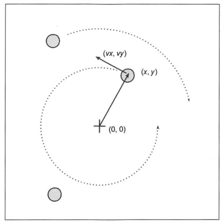
为了模拟这个运动，我们需要如下信息：粒子的起始位置、速度和旋转方向。因此定义一个通用的Particle类，用于存储粒子的位置及角速度。

class Particle:
    def __init__(self, x, y, ang_vel):
        self.x = x
        self.y = y
        self.ang_vel = ang_vel

  对于特定粒子，经过时间t后，它将到达圆周上的下一个位置。我们可以这样近似计算圆周轨迹：将时间段t分成一系列很小的时间段dt，在这些很小的时段内，粒子沿圆周的切线移动。这样就近似模拟了圆周运动。粒子运动方向可以按照下面的公式计算：

v_x = -y / (x **2 + y **2) ** 0.5
v_y = x / (x **2 + y **2) ** 0.5

  计算经过时间t后的粒子位置，必须采取如下步骤：

1）计算运动方向（v_x和v_y)

2）计算位置(d_x和d_y)，即时段dt、角速度和移动方向的乘积

3）不断重复第1步和第2步，直到时间过去t

class ParticleSimulator:
    def __init__(self, particles):
        self.particles = particles

    def evolve(self, dt):
        timestep = 0.00001
        nsteps = int(dt / timestep)

        for i in range(nsteps):
            for p in self.particles:
                norm = (p.x **2 + p.y ** 2) ** 0.5
                v_x = -p.y / norm
                v_y = p.x / norm

                d_x = timestep * p.ang_vel * v_x
                d_y = timestep * p.ang_vel * v_y

                p.x += d_x
                p.y += d_y

  下面就是进行绘图了，我们先把代码放上来，再具体解释：

def visualize(simulator):
    X = [p.x for p in simulator.particles]
    Y = [p.y for p in simulator.particles]

    fig = plt.figure()
    ax = plt.subplot(111, aspect = 'equal')
    line, = ax.plot(X, Y, 'ro')  #如果不加逗号，返回值是包含一个元素的list，加上逗号表示直接将list的值取出

    plt.xlim(-1, 1)
    plt.ylim(-1, 1)

    def init():
        line.set_data([], [])
        return line,   #加上逗号表示返回包含只元素line的元组

    def animate(i):
        simulator.evolve(0.01)
        X = [p.x for p in simulator.particles]
        Y = [p.y for p in simulator.particles]

        line.set_data(X, Y)
        return line,   #加上逗号表示返回包含只元素line的元组

    anim = animation.FuncAnimation(fig,
                                   animate,
                                   init_func = init,
                                   blit = True,
                                   interval = 10)
    plt.show()

这里再对animation.FuncAnimation函数作具体解释：

• fig表示动画绘制的画布
• func = animate表示绘制动画，本例中animate的参数未使用，但不可省略
• frames参数省略未写，表示要传给func的参数，省略的话会一直累加
• blit表示是否更新整张图
• interval表示更新频率，单位为ms

完整代码如下:

# -*- coding: utf-8 -*-

from matplotlib import pyplot as plt
from matplotlib import animation
import numpy as np

class Particle:
    def __init__(self, x, y, ang_vel):
        self.x = x
        self.y = y
        self.ang_vel = ang_vel

class ParticleSimulator:
    def __init__(self, particles):
        self.particles = particles

    def evolve(self, dt):
        timestep = 0.00001
        nsteps = int(dt / timestep)

        for i in range(nsteps):
            for p in self.particles:
                norm = (p.x **2 + p.y ** 2) ** 0.5
                v_x = -p.y / norm
                v_y = p.x / norm

                d_x = timestep * p.ang_vel * v_x
                d_y = timestep * p.ang_vel * v_y

                p.x += d_x
                p.y += d_y


def visualize(simulator):
    X = [p.x for p in simulator.particles]
    Y = [p.y for p in simulator.particles]

    fig = plt.figure()
    ax = plt.subplot(111, aspect = 'equal')
    line, = ax.plot(X, Y, 'ro')

    plt.xlim(-1, 1)
    plt.ylim(-1, 1)

    def init():
        line.set_data([], [])
        return line,

    def init2():
        line.set_data([], [])
        return line

    def animate(aa):
        simulator.evolve(0.01)
        X = [p.x for p in simulator.particles]
        Y = [p.y for p in simulator.particles]

        line.set_data(X, Y)
        return line,

    anim = animation.FuncAnimation(fig,
                                   animate,
                                   frames=10,
                                   init_func = init,
                                   blit = True,
                                   interval = 10)
    plt.show()


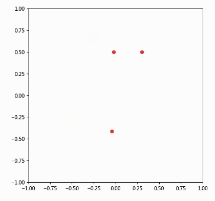
def test_visualize():
    particles = [Particle(0.3, 0.5, 1),
                 Particle(0.0, -0.5, -1),
                 Particle(-0.1, -0.4, 3)]
    simulator = ParticleSimulator(particles)
    visualize(simulator)

if __name__ == '__main__':
    test_visualize()

绘制效果如下：

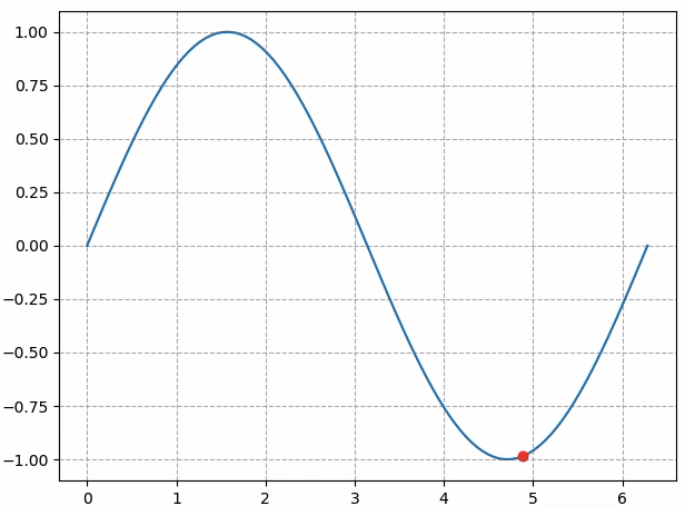
  可能很多同学看了上面这个例子，也不是很清楚animation函数的用法，下面我们再举个简单例子：

import numpy as np
import matplotlib
import matplotlib.pyplot as plt
import matplotlib.animation as animation
 
def update_points(num):
    point_ani.set_data(x[num], y[num])
    return point_ani,
 
x = np.linspace(0, 2*np.pi, 100)
y = np.sin(x)
 
fig = plt.figure(tight_layout=True)
plt.plot(x,y)
point_ani, = plt.plot(x[0], y[0], "ro")
plt.grid(ls="--")

ani = animation.FuncAnimation(fig, update_points, frames = np.arange(0, 100), interval=100, blit=True)
 
plt.show()

显示效果如下图所示：

但如果把animation.FuncAnimation中的frames参数改成`np.arange(0, 10):

ani = animation.FuncAnimation(fig, update_points, frames = np.arange(0, 10), interval=100, blit=True)

那显示效果就会如下图所示：

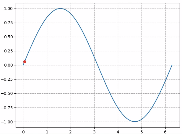
这是因为我们定义了一百个点的数据，但只看前10个点。

微信公众号：Quant_Times