深入理解Detectron 2 — Part5 ROI (Box) Head

之前我们已经介绍了基础网络架构和代码库结构，特征金字塔网络， 数据加载器和Ground Truth实例,区域建议网络（Region Proposal Network） 。本篇文章,我们将深入研究整个pipeline的最后一部分——ROI (Box) Head³（见图 2）。

Figure 2. Detailed architecture of Base-RCNN-FPN. Blue labels represent class names.

 在 ROI (Box) Head，我们将 a) 来自 FPN 的特征图，b) 提议框（proposal boxes）和 c) 真实框作为输入（ground truth boxes）。

a) 来自 FPN 的特征图

正如我们在特征金字塔网络中看到的，来自 FPN 的输出特征图是：

output[“p2”].shape -> torch.Size([1, 256, 200, 320]) # stride = 4 
output[“p3”].shape -> torch.Size([1, 256, 100, 160]) # stride = 8
output[“p4”].shape -> torch.Size([1, 256, 50, 80]) # stride = 16
output[“p5”].shape -> torch.Size([1, 256, 25, 40]) # stride = 32
output[“p6”].shape -> torch.Size([1, 256, 13, 20]) # stride = 64

每个张量大小代表（批次、通道、高度、宽度）。我们在整个博客系列中使用上述特征维度。 P2-P5 特征被送到ROI (Box) Head，P6 未被使用。

b) 提案框（proposal boxes）被包含在来自 RPN（参见区域建议网络（Region Proposal Network））的输出实例中，它们具有 1000 个“proposal_boxes”和 1000 个“objectness_logits”。在 ROI Heads 中，仅使用了proposal box 来裁剪特征图并处理 ROIs，并且不使用 objectness_logits。

{'proposal_boxes': 
    Boxes(tensor([[675.1985, 469.0636, 936.3209, 695.8753],
                  [301.7026, 513.4204, 324.4264, 572.4883],
                  [314.1965, 448.9897, 381.7842, 491.7808],
               ...,
'objectness_logits': 
    tensor([ 9.1980,  8.0897,  8.0897, ...]
}

c) 从数据集中加载了标注的真实框（参考 数据加载器和Ground Truth实例）

'gt_boxes': Boxes(tensor([
[100.55, 180.24, 114.63, 103.01],
[180.58, 162.66, 204.78, 180.95]
])),
'gt_classes': tensor([9, 9])

图 3 显示了 ROI Heads 的详细示意图。所有计算都在 Detectron 2 中的 GPU 上执行。

Figure 3. Schematic of ROI Heads. Blue and red labels represent class names and chapter titles respectively.

1. 推荐框（Proposal Box） 采样（仅在训练期间）

在 RPN 中，我们从 FPN 五个级别（P2 到 P6）的输出特征中获得了 1,000 个推荐框。推荐框用于从特征图中裁剪感兴趣的区域 (ROI)，这些区域被馈送到 Box Head。为了加速训练，我们在预测的推荐框中添加了真实框。例如，如果图像有两个真实框（ ground truth box)，则推荐区域总数将为 1002。

在训练过程中，前景和背景推荐框首先被重新采样以平衡训练目标数量。

使用 Matcher 将 IoU 高于阈值的推荐框设为前景，将其他推荐框设为背景（见图 4）。请注意，与 RPN 不同，在 ROI Heads 中没有“忽略”框。添加的真实框与自身完美匹配（IoU 100%），因此被视为前景。

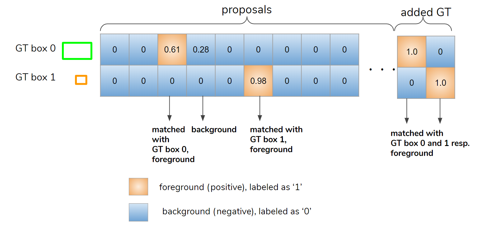
Figure 4. Matcher determines assignment of anchors to ground-truth boxes. The table shows the IoU matrix whose shape is (number of GT boxes, number of anchors).

接下来，我们平衡前景框和背景框的数量。设 N 为（前景 + 背景）框的目标数量，F 为前景框的目标数量。 N 和 F/N 由以下配置参数定义。框的采样如图 5 所示，以便前景框的数量小于 F。

N: MODEL.ROI_HEADS.BATCH_SIZE_PER_IMAGE (typically 512)
F/N: MODEL.ROI_HEADS.POSITIVE_FRACTION (typically 0.25)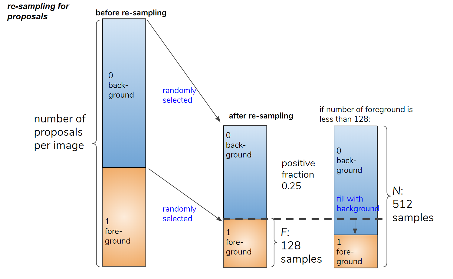

Figure 5. Re-sampling the foreground and background proposal boxes.

2. ROI 池化（Pooling）

在ROI 池化过程中，需要裁剪（或池化）由推荐框指定的特征图的矩形区域。

级别分配

假设我们有两个推荐框（图 6 中的灰色和蓝色矩形）和P2 到 P5的特征图，如图6所示。

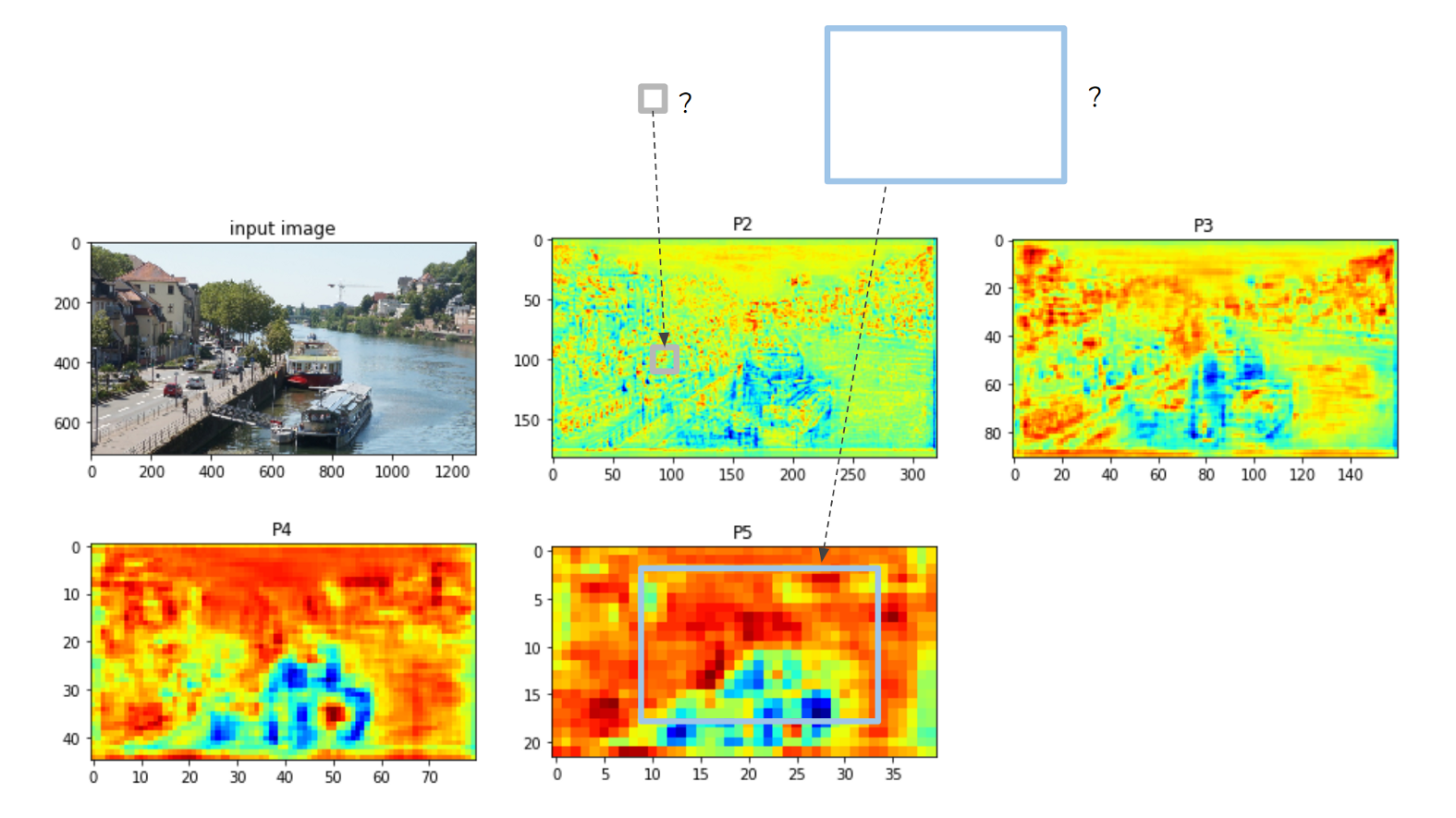
Figure 6. feature level assignment of proposal boxes for ROI pooling.

对于两个特征框中的任意一个框，应该从哪个特征图裁剪 ROI？如果将小灰色框分配给 P5 特征，则该框内将仅包含一两个特征像素，因此将丢失很多特征。

有一个规则可以将提议框分配给适当的特征图：

指定的特征级别算法：floor(4 + log2(sqrt(box_area) / 224))

其中 224 是推荐框大小。例如，如果proposal box的大小为224×224，则分配到第4层（P4）。

在图 6 的情况下，灰色框分配给 P2 层，蓝色框分配给 P5层。级别分配在assign_boxes_to_levels 函数中处理。

ROIAlignV2

为了准确裁剪 ROI（具有浮点坐标的推荐框），Mask R-CNN 论文⁴中提出了一种称为 ROIAlign 的方法。在 Detectron 2 中，默认的池化方法称为 ROIAlignV2，它是 ROIAlign 的略微修改版本。

在图 7 中，描绘了 ROIAlignV2 和 ROIAlign。大矩形是 ROI 中的一个 bin（或像素）。为了汇集（pool）矩形内的特征值，放置了四个采样点来插入四个相邻的像素值。最终的 bin 值是通过平均四个采样点值来计算的。 ROIAlignV2 和 ROIAlign 的区别很简单。从 ROI 坐标中减去半像素偏移 (0.5) 以更准确地计算相邻像素索引。详情请看图7。

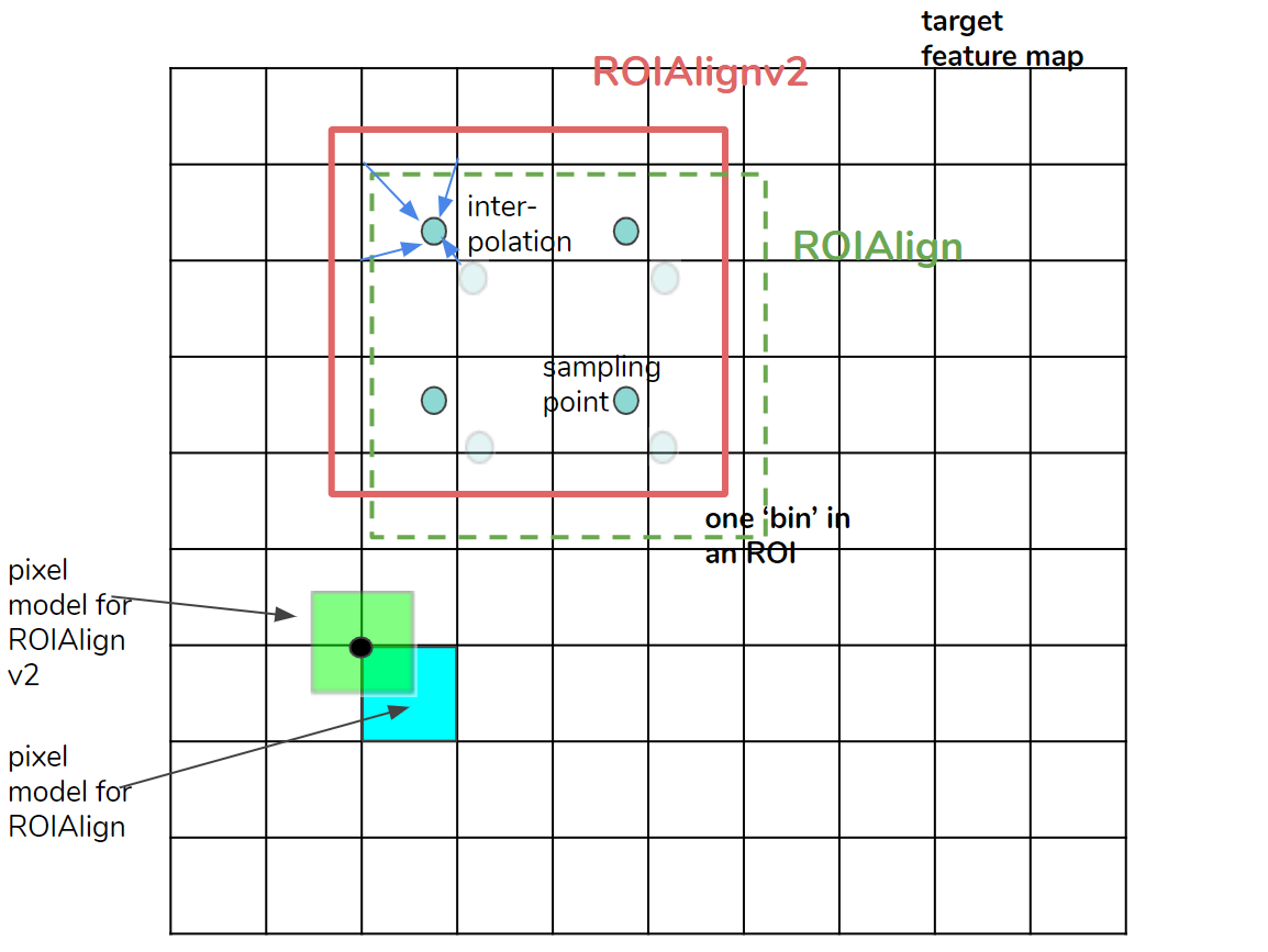
Figure 7. ROIAlignv2. Compared with ROIAlign(v1), the half-pixel offset (0.5) is subtracted from ROI coordinates to compute neighboring pixel indices more accurately. ROIAlignV2 employs the pixel model in which pixel coordinates represent the centers of pixels.

现在通过 ROIAlignV2 从相应的级别 (P2-P5) 裁剪 ROI。生成的张量的大小为：

[B, C, H, W] = [N × batch size, 256, 7, 7]

其中 B、C、H 和 W 分别代表batch中的 ROI 数、通道数、高度和宽度。默认情况下，对于一个batch，ROI 数N为 512，ROI 大小为 7 × 7。张量是裁剪实例特征的集合，其中包括平衡的前景和背景 ROI。

3. Box Head

在 ROI Pooling 之后，裁剪后的特征被馈送到头部网络。至于Mask R-CNN⁴，有两种Head：box head和mask head。然而，Base R-CNN FPN 只有称为 FastRCNNConvFCHead 的box头，它对 ROI 内的对象进行分类并微调盒的位置和形状。

Box Head 默认的网络层如下：

(box_head): FastRCNNConvFCHead(
      (fc1): Linear(in_features=12544, out_features=1024, bias=True)
      (fc2): Linear(in_features=1024, out_features=1024, bias=True)
    )
(box_predictor): FastRCNNOutputLayers(
      (cls_score): Linear(in_features=1024, out_features=81, bias=True)
      (bbox_pred): Linear(in_features=1024, out_features=320, bias=True)

如您所见，头部不包含任何卷积层。
大小为 [B, 256, 7, 7] 的输入张量被展平为 [B, 256×7 ×7 = 12,544 个通道]，以馈送到全连接 (FC) 层 1 (fc1)。
在两个 FC 层之后，张量到达最后的 box_predictor 层：cls_score（线性）和 bbox_pred（线性）。
最后一层的输出张量是：

cls_score -> scores             # shape:(B, 80+1)
bbox_pred -> prediction_deltas  # shape:(B, 80×4)

接下来我们看看如何计算训练期间输出的损失。

4. Loss 计算(仅仅在训练期间)

两个损失函数应用于最终输出张量。

位置 loss (loss_box_reg)

• l1 loss⁵.

• foreground predictions are picked from the pred_proposal_deltas 张量，其shape 是 (N samples × batch size, 80×4). 例如, 如果第15个样本是类别索引为17的前景, the indices of [14 (=15–1), [68 (=17×4), 69, 70, 71]] 被选择.
• foreground ground truth targets are picked from gt_proposal_deltas，其 shape 是 (B, 4). The tensor values are the relative sizes of the ground truth boxes compared with the proposal boxes, which are calculated by the Box2BoxTransform.get_deltas function (see section 3–3 of Part4). The tensor with foreground indices are sampled from gt_proposal_deltas.

分类 loss (loss_cls)

• Softmax 交叉熵损失
• 计算所有前景和背景预测分数 [B, K 类] vs 真实标签类索引[B]
• 分类目标是所有的前景类和背景类，因此 K = 种类数 + 1（COCO 数据集的背景类索引为“80”）。

{
'loss_cls': tensor(4.3722, device='cuda:0', grad_fn=<NllLossBackward>),
 'loss_box_reg': tensor(0.0533, device='cuda:0', grad_fn=<DivBackward0>)
}

5. Inference（仅仅在测试时）

正如我们在第 3 节中看到的，我们有形状为 (B, 80+1) 的预测分数和形状为 (B, 80×4) 的 predict_deltas（预测增量） 作为 Box Head 的输出

1.将预测增量（prediction deltas）应用于推荐框

为了计算最终的预测框坐标，这里使用到了预测增量 prediction deltas⁶ : Δx, Δy, Δw, 和Δh, 并且用到了Box2BoxTransform.apply_deltas (Fig. 8). 这个与 as the step 1 in the section 5 of Part 4一样.

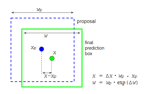
  Figure 8. applying prediction deltas to a proposal box to calculate the coordinates of the final prediction box.

2. 按预测得分过滤预测框

我们首先过滤掉低分的边界框，如下所示图 9 中的 n（从左到中）。每个框都有相应的分数，因此很容易做到这一点。

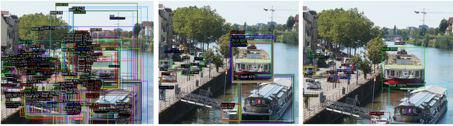
Figure 9. Post-processing at the inference stage. left: visualization of all the ROIs before post-processing. center: after score thresholding. right: after non-maximum suppression.

 3. 非最大比抑制（non-maximum suppression）

为了去除重叠框，应用了非最大抑制（NMS）（图 9，中到右）。 NMS 的参数定义在这里。

4. 选择前 k 个结果

最后，当剩余框的数量大于预定义的数量时，我们选择前 k 个结果。

[1] This is a personal article and the opinions expressed here are my own and not those of my employer.
[2] Yuxin Wu, Alexander Kirillov, Francisco Massa, Wan-Yen Lo and Ross Girshick, Detectron2. GitHub - facebookresearch/detectron2: Detectron2 is FAIR's next-generation platform for object detection, segmentation and other visual recognition tasks., 2019. The file, directory, and class names are cited from the repository ( Copyright 2019, Facebook, Inc. )
[3] the files used for ROI Heads are: modeling/roi_heads/roi_heads.py, modeling/roi_heads/box_head.py, modeling/roi_heads/fast_rcnn.py, modeling/box_regression.py, modeling/matcher.py and modeling/sampling.py .
[4] Kaiming He, Georgia Gkioxari, Piotr Dollar, and Ross Girshick. Mask R-CNN. In ICCV, 2017.
[5] Implemented as smooth-l1 loss, but it’s actually used as pure-l1 loss unlike Detectron1 or MMDetection. (see : link).
[6] Shaoqing Ren, Kaiming He, Ross Girshick, and Jian Sun. Faster R-CNN: Towards real-time object detection with region proposal networks. In NIPS, 2015. (link)Digging into Detectron 2 — part 5 | by Hiroto Honda | Medium