


 平场校正是一种用于图像传感器的校正技术,通过消除传感器响应不均匀性和光照差异导致的图像质量下降。它涉及获取不同条件下的图像(如均匀光、暗场等),然后通过数学运算来校正图像,提高亮度均匀性和减少伪影。此过程通常应用于工业相机,而在消费级设备中,校正可能在硬件级别已完成。
什么是平场校正
平场校正(Flat Field Correction),也称为光场校正、灰度校正或散斑校正,是一种用于图像传感器或相机校正的图像处理技术。它旨在消除图像中由于传感器不均匀响应、光照差异或其他因素引起的亮度和颜色不均匀性。平场校正可以提高图像的质量,使得不同区域的亮度更加均匀,减少了图像中的伪影、噪声和其他影响。
平场校正的主要思想是使用一个称为“平场图像”或“平场图”(Flat Field Image)的参考图像,该图像是由一个均匀光源照射到传感器上所得到的。平场图像捕捉了传感器的响应非均匀性,以及在不同区域的光照差异。
矫正原理过程
第一步,获取四幅图像
D
light
D_{\text {light}}
Dlight,
D
dark
D_{\text {dark}}
Ddark,
D
s-light
D_{\text {s-light}}
Ds-light,
D
s-dark
D_{\text {s-dark}}
Ds-dark
D
light
D_{\text {light}}
Dlight 为均匀光下,感光芯片拍摄的图片
D
dark
D_{\text {dark}}
Ddark 为无光下,感光芯片拍摄的图片
D
s-light
D_{\text {s-light}}
Ds-light 为正常情况下(有各种物体遮挡光源等非均匀光),感光芯片拍摄的图片
D
s-dark
D_{\text {s-dark}}
Ds-dark 为正常情况下无光下,感光芯片拍摄的图片
对于感光器件,所采集到的图片符合如下公式:
D
=
G
(
x
,
y
)
I
(
x
,
y
)
+
Q
D=G_{(x, y)} I_{(x, y)}+Q
D=G(x,y)I(x,y)+Q
其中
D
D
D为感光后的图片数据,
G
(
x
,
y
)
G_{(x, y)}
G(x,y)为感光器件的增益,一般为线性的,
I
(
x
,
y
)
I_{(x, y)}
I(x,y)则为光强,
Q
Q
Q则为噪声,主要包括读出随机噪声
Q
1
Q_1
Q1,读出电路引入的FPN噪声
Q
2
Q_2
Q2,初始阈值不一致引入的FPN噪声
Q
3
Q_3
Q3,光散粒噪声
Q
4
Q_4
Q4以及器件光响应不一致引入的FPN噪声
Q
5
Q_5
Q5。其中FPN噪声是影响成像质量的关键因素,因此我们引入均场矫正的方法来消弱图像的FPN噪声。
D
light
=
G
(
x
,
y
)
I
0
+
Q
(
1
)
D_{\text {light}} = G_{(x, y)} I_{0}+Q\space(1)
Dlight=G(x,y)I0+Q (1)
D
dark
=
G
(
x
,
y
)
∗
0
+
Q
=
Q
(
2
)
D_{\text {dark}} = G_{(x, y)}* 0+Q =Q\space(2)
Ddark=G(x,y)∗0+Q=Q (2)
D
light
−
D
dark
=
G
(
x
,
y
)
I
0
(
3
)
D_{\text {light}} - D_{\text {dark}}= G_{(x, y)} I_{0}\space(3)
Dlight−Ddark=G(x,y)I0 (3)
这里通过
D
light
−
D
dark
D_{\text {light}} - D_{\text {dark}}
Dlight−Ddark消除了噪声
Q
Q
Q,当然这里只是消除了前述的FPN噪声,包括读出电路引入的FPN噪声
Q
2
Q_2
Q2,初始阈值不一致引入的FPN噪声
Q
3
Q_3
Q3,器件光响应不一致引入的FPN噪声
Q
5
Q_5
Q5,并没有消除读出随机噪声
Q
1
Q_1
Q1和光散粒噪声
Q
4
Q_4
Q4。由于
Q
1
Q_1
Q1和
Q
4
Q_4
Q4影响较小,所以忽略不计了。
D
light-sample
=
G
(
x
,
y
)
I
(
x
,
y
)
+
Q
(
4
)
D_{\text {light-sample}} = G_{(x, y)} I_{(x,y)}+Q\space(4)
Dlight-sample=G(x,y)I(x,y)+Q (4)
D
dark-sample
=
G
(
x
,
y
)
∗
0
+
Q
=
Q
(
5
)
D_{\text {dark-sample}} = G_{(x, y)}* 0+Q =Q\space(5)
Ddark-sample=G(x,y)∗0+Q=Q (5)
D
light-sample
−
D
dark-sample
=
G
(
x
,
y
)
I
(
x
,
y
)
(
6
)
D_{\text {light-sample}} - D_{\text {dark-sample}}= G_{(x, y)} I_{(x,y)}\space(6)
Dlight-sample−Ddark-sample=G(x,y)I(x,y) (6)
第二步,用公式3和6直接相比,可以消除增益
G
(
x
,
y
)
G_{(x, y)}
G(x,y)
D
c
=
D
s
−
light
−
D
s
−
d
a
r
κ
D
light
−
D
darr
∗
k
=
G
(
x
,
y
)
I
(
x
,
y
)
G
(
x
,
y
)
I
0
∗
k
(
7
)
D_c=\frac{D_{s-\text { light }}-D_{s-d a r \kappa}}{D_{\text {light }}-D_{\text {darr }}} * k=\frac{G_{(x, y)} I_{(x, y)}}{G_{(x, y)} I_0}*k\space(7)
Dc=Dlight −Ddarr Ds− light −Ds−darκ∗k=G(x,y)I0G(x,y)I(x,y)∗k (7)
D c = k I 0 ∗ I ( x , y ) ( 8 ) D_c=\frac{k}{I_0} * I_{(x, y)}\space(8) Dc=I0k∗I(x,y) (8)
此时,所有像素的光响应增益均等效为 k I 0 \frac{k}{I_0} I0k ,为一个近似的常数,这样得到的 D c D_c Dc只和关照的场强有关,当然这是一个理想结果,但在实际应用中由于Q_1和Q_4以及非理想均匀光I_0等各种因素的存在,FPN噪声不可能完全消除只能一定程度改善。
以上是平场矫正的原理。
什么时候进行均场矫正
我们的手机还有照相机为何从来没有平场矫正?
因为在电路级别已经做过了。
而一般的工业相机,可能需要定期做平场矫正。
代码实现
def Flat_Field_Correction():
dark = cv2.imread('C:\\Users\\Administrator\\Desktop\\test\\BMP20230816_172727.bmp', cv2.IMREAD_GRAYSCALE)[5000:5640,5000:5640]
raw = cv2.imread('C:\\Users\\Administrator\\Desktop\\test\\BMP20230816_172634.bmp', cv2.IMREAD_GRAYSCALE)[5000:5640,5000:5640]
flat_dark = cv2.imread('C:\\Users\\Administrator\\Desktop\\test\\D1.bmp', cv2.IMREAD_GRAYSCALE)[5000:5640,5000:5640]
flat_light = cv2.imread('C:\\Users\\Administrator\\Desktop\\test\\l1.bmp', cv2.IMREAD_GRAYSCALE)[5000:5640,5000:5640]
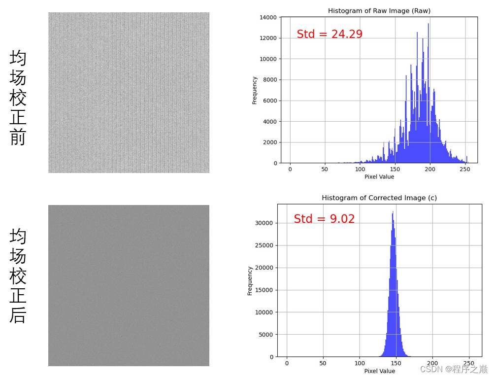
m = np.average(np.abs(raw-dark))
c = ((np.abs(raw-dark))/(np.abs(flat_light-flat_dark)))*m
cv2.imwrite('c.bmp',c)
cv2.imwrite('raw.bmp', raw)
# hist, bins = np.histogram(raw.flatten(), bins=256, range=(0, 255))
std_deviation = np.std(raw.flatten())
# 绘制直方图
plt.figure()
plt.hist(raw.flatten(), bins=256, range=(0, 255), color='blue', alpha=0.7)
plt.xlabel('Pixel Value')
plt.ylabel('Frequency')
plt.title('Histogram of Raw Image (Raw)')
plt.grid(True)
figtext_x = 10 # 调整文本位置的x坐标(0.85表示右上角)
figtext_y = 12000 # 调整文本位置的y坐标(0.9表示上方略下)
# 在图中标注标准差的值
plt.text(figtext_x, figtext_y, 'Std = {:.2f}'.format(std_deviation), fontsize=20, color='red')
# plt.show()
plt.savefig('raw_result.jpg')
# 计算直方图的标准差
# 计算直方图
# hist, bins = np.histogram(c.flatten(), bins=256, range=(0, 255))
std_deviation = c.flatten().astype('int8').std()
# 绘制直方图
plt.figure()
plt.hist(c.flatten(), bins=256, range=(0, 255), color='blue', alpha=0.7)
plt.xlabel('Pixel Value')
plt.ylabel('Frequency')
plt.title('Histogram of Corrected Image (c)')
plt.grid(True)
figtext_x = 10 # 调整文本位置的x坐标(0.85表示右上角)
figtext_y = 30000 # 调整文本位置的y坐标(0.9表示上方略下)
# 在图中标注标准差的值
plt.text(figtext_x, figtext_y, 'Std = {:.2f}'.format(std_deviation), fontsize=20, color='red')
# plt.show()
plt.savefig('corrected_result.jpg')


 3529
3529

 被折叠的 条评论
为什么被折叠?
被折叠的 条评论
为什么被折叠?
 到【灌水乐园】发言


