


开发环境
作者:嘟粥yyds
时间:2023年7月14日
集成开发工具:Google Colab
集成开发环境:Python 3.10.6
第三方库:tensorflow、tensorflow_datasets、tensorflow_hub、matplotlib、textwrap、numpy、time
概要
实现具有视觉注意力的图像描述,本文要点如下:
- 了解如何创建图像描述模型
- 了解如何训练和预测文本生成模型。
图像描述模型将图像作为输入,并输出文本。理想情况下,我们希望模型的输出能够准确描述图像中的事件/事物,类似于人类可能提供的描述。
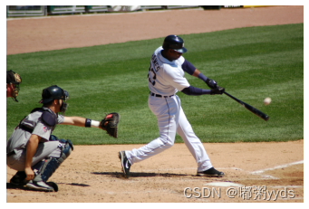
例如,给定如下例所示的图像,模型预计将生成诸如“有些人正在打棒球。”的标题。
为了生成文本,我们构建了一个编码器-解码器模型,其中编码器输出输入图像的嵌入,解码器从图像嵌入中输出文本
本文将使用类似于Show, Attend and Tell: Neural Image Caption Generation with Visual Attention的模型架构,并构建基于注意力的图像描述模型。
本文使用的训练集为COCO大规模目标检测、分割、描述数据集。
实现步骤
1 导入TensorFlow和其他所需库
import time
from textwrap import wrap  # 用于对文本进行换行处理

import matplotlib.pylab as plt
import numpy as np
import tensorflow as tf
import tensorflow_datasets as tfds
import tensorflow_hub as hub
from tensorflow.keras import Input
from tensorflow.keras.layers import (
    GRU,
    Add,
    AdditiveAttention,
    Attention,
    Concatenate,
    Dense,
    Embedding,
    LayerNormalization,
    Reshape,
    StringLookup,
    TextVectorization,
)

print(tf.version.VERSION)
2 读取和准备数据集
我们将使用TensorFlow数据集功能来读取COCO标题数据集。
此版本包含来自COCO 2014的图像、边界框、标签和描述,分为Karpathy和Li(2015)定义的子集,并采用处理原始数据集的一些数据质量问题(例如,一些原始数据集中的图像没有标题)
首先,让我们定义一些常量。
本文使用的是来自 tf.keras.applications 的预训练InceptionResNetV2模型作为特征提取器,因此一些常量来自InceptionResNetV2模型定义。如果您想使用其他类型的基本模型,请确保也更改这些常数。
tf.keras.applications是一个预训练的模型存储库,类似于TensorFlow Hub,虽然Tensorflow Hub托管不同模式的模型,包括图像、文本、音频等,但tf.keras.application仅托管流行且稳定的图像模型。
相比之下,tf.keras.applications更灵活,因为它包含模型元数据,允许我们访问和控制模型行为,而大多数基于TensorFlow Hub的模型只包含编译后的SavedModels。
# 改变这些以控制精度/速度
VOCAB_SIZE = 20000  # 定义词汇表的大小,限制用于训练模型的单词数量。该值越小则模型收敛速度越快
ATTENTION_DIM = 512  # 指定注意力层中密集层的维度
WORD_EMBEDDING_DIM = 128  # 指定词嵌入向量的维度

# InceptionResNetV2 将(299, 299, 3)的图像作为输入并且返回(8, 8, 1536)
# 定义特征提取器模型
FEATURE_EXTRACTOR = tf.keras.applications.inception_resnet_v2.InceptionResNetV2(
    include_top=False, weights="imagenet"
)
IMG_HEIGHT = 299
IMG_WIDTH = 299
IMG_CHANNELS = 3
FEATURES_SHAPE = (8, 8, 1536)
3 过滤和预处理
在这里,我们对数据集进行预处理。下面的函数:
- 将图像调整为(
IMG_HEIGHT,IMG_WIDTH)形状 - 重新调整像素值从[0, 255]到[0, 1]
- 返回图像(
image_tensor)和描述(captions)字典。
注意:此数据集太大,无法存储在本地环境中。因此,它存储在位于us-Cental1的公共GCS存储桶中。如果您从美国以外的笔记本电脑访问它,它将速度很慢并且需要支付网络费用。
# 定义数据集所在的Google云存储(GCS)路径。
GCS_DIR = "gs://asl-public/data/tensorflow_datasets/"
BUFFER_SIZE = 1000  # 定义数据集中用于缓冲和随机化的样本数。该值越大,随机化程度越高。


def get_image_label(example):
  """
  处理数据集中的每个样本。接收一个样本作为输入,从中提取图像和标签信息,并进行预处理。
  返回包含图像张量和标题的字典
  """
  caption = example["captions"]["text"][0]  # 每张图片只有第一个标题
  img = example["image"]
  img = tf.image.resize(img, (IMG_HEIGHT, IMG_WIDTH))
  img = img / 255

  return {"image_tensor": img, "caption": caption}

# 加载数据集的训练集部分
trainds = tfds.load("coco_captions", split="train", data_dir=GCS_DIR)
# 对训练集中的每个样本映射为包含图像张量和标题的字典。
trainds = trainds.map(
    get_image_label, num_parallel_calls=tf.data.AUTOTUNE  # 使用自动调整并行处理
).shuffle(BUFFER_SIZE)

# 使用prefetch函数对训练集数据进行预取,以提高数据加载的效率。
trainds = trainds.prefetch(buffer_size=tf.data.AUTOTUNE)
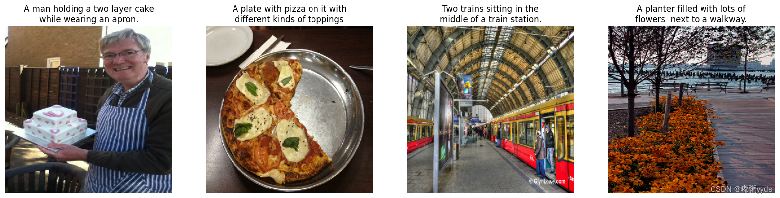
4 可视化
让我们看一下数据集中的图像和示例标题。
f, ax = plt.subplots(1, 4, figsize=(20, 5))
for idx, data in enumerate(trainds.take(4)):
  ax[idx].imshow(data["image_tensor"].numpy())
  # 获取当前样本的标题,并将标题文本进行换行处理。即当字符串超过宽度30时进行换行
  caption = "\n".join(wrap(data["caption"].numpy().decode("utf-8"), 30))
  ax[idx].set_title(caption)
  ax[idx].axis("off")
plt.show()  # 显示图形
5 文本预处理
我们添加特殊的标记来表示句子的开始(<start>)和结束(<end>)。
这里添加了开始和结束标记,因为我们使用编码器-解码器模型,在预测期间,为了开始描述,我们使用<start>,并且由于描述长度可变,我们在看到<end>标记时终止预测。
然后创建标题的完整列表以供进一步预处理。
def add_start_end_token(data):
    start = tf.convert_to_tensor("<start>")
    end = tf.convert_to_tensor("<end>")
    data["caption"] = tf.strings.join(
        [start, data["caption"], end], separator=" "
    )
    return data


trainds = trainds.map(add_start_end_token)
6 预处理和标记标题
本文使用的是TextVectoration层将文本标题转换为整数序列,步骤如下:
- 使用adapt遍历所有标题,将标题拆分为单词,并计算顶部
VOCAB_SIZE单词的词汇表。 - 通过将每个单词映射到词汇表中的索引来标记所有描述。所有输出序列都将填充到长度
MAX_CAPTION_LEN。这里我们直接指定64,这对于这个数据集来说已经足够了,但是请注意,如果您不想减少数据集中很长的句子,这个值应该通过处理整个数据集来计算。
注意:此过程大约需要8分钟。
# 定义标题文本的最大长度
MAX_CAPTION_LEN = 64


# 我们将覆盖TextVectoration的默认标准化以保留
# "<>" 字符,因此我们保留<start>和<end>的标记。
def standardize(inputs):
  """
  标准化文本数据。接收一个文本输入inputs,将其转换为小写并移除标点符号等特殊字符。
  """
  inputs = tf.strings.lower(inputs)
  return tf.strings.regex_replace(
      inputs, r"[!\"#$%&\(\)\*\+.,-/:;=?@\[\\\]^_`{|}~]?", ""
  )


# 从词汇表中选择最常用的单词并删除标点符号等。
tokenizer = TextVectorization(
  max_tokens=VOCAB_SIZE,
  standardize=standardize,
  output_sequence_length=MAX_CAPTION_LEN,
)

# 使用adapt函数将文本向量化器适应到训练数据集中的标题文本
tokenizer.adapt(trainds.map(lambda x: x["caption"]))
让我们尝试标记示例文本
tokenizer(["<start> This is a sentence <end>"])
"""输出如下:
<tf.Tensor: shape=(1, 64), dtype=int64, numpy=
array([[  3, 165,  11,   2,   1,   4,   0,   0,   0,   0,   0,   0,   0,
          0,   0,   0,   0,   0,   0,   0,   0,   0,   0,   0,   0,   0,
          0,   0,   0,   0,   0,   0,   0,   0,   0,   0,   0,   0,   0,
          0,   0,   0,   0,   0,   0,   0,   0,   0,   0,   0,   0,   0,
          0,   0,   0,   0,   0,   0,   0,   0,   0,   0,   0,   0]])>
"""
遍历训练数据集中的前3个样本,并将它们的标题文本提取出来。方便地查看和检查训练数据集中的一些样本标题文本,以确保数据的正确性和一致性。
sample_captions = []
for d in trainds.take(3):
  sample_captions.append(d["caption"].numpy())

sample_captions
[b'<start> A man is cupping his hand near his mouth while standing in front of a group of cows in the background in a pasture.  <end>',
 b'<start> a plane flying through the air over some mountains  <end>',
 b'<start> A skater holding a trick on his board at a skate park <end>']
print(tokenizer(sample_captions))
"""输出如下:
tf.Tensor(
[[   3    2   12   11 6542   50  187   46   50  375   56   15    8   38
     5    2   31    5  244    8    7  178    8    2  619    4    0    0
     0    0    0    0    0    0    0    0    0    0    0    0    0    0
     0    0    0    0    0    0    0    0    0    0    0    0    0    0
     0    0    0    0    0    0    0    0]
 [   3    2  197   74   96    7  118   88   36  525    4    0    0    0
     0    0    0    0    0    0    0    0    0    0    0    0    0    0
     0    0    0    0    0    0    0    0    0    0    0    0    0    0
     0    0    0    0    0    0    0    0    0    0    0    0    0    0
     0    0    0    0    0    0    0    0]
 [   3    2 2296   26    2  303    6   50  120   21    2  253  141    4
     0    0    0    0    0    0    0    0    0    0    0    0    0    0
     0    0    0    0    0    0    0    0    0    0    0    0    0    0
     0    0    0    0    0    0    0    0    0    0    0    0    0    0
     0    0    0    0    0    0    0    0]], shape=(3, 64), dtype=int64)
 """
请注意,所有句子都以相同的标记开始和结束(例如“3”和“4”)。这些值分别表示开始标记和结束标记。
您还可以将id转换为原始文本。
for wordid in tokenizer([sample_captions[0]])[0]:
  print(tokenizer.get_vocabulary()[wordid], end=" ")
"""输出如下:
<start> a man is cupping his hand near his mouth while standing in front of a group of cows in the background in a pasture <end>
"""
此外,我们可以使用StringLookup层创建Word<->索引转换器。
# 查找表:单词->索引
word_to_index = StringLookup(
  mask_token="", vocabulary=tokenizer.get_vocabulary()
)

# 查找表:索引->单词
index_to_word = StringLookup(
    mask_token="", vocabulary=tokenizer.get_vocabulary(), invert=True
)
7 为训练创建tf.data数据集
现在让我们将调整后的标记化应用于所有样本,并创建tf.data数据集进行训练。
请注意,我们还通过从功能标题中转移文本来创建标签。
如果我们有一个输入标题"<start> I love cats <end>",它的标签应该是"I love cats <end> <padding>"。
有了这个,我们的模型可以尝试从<start>学习预测I。
数据集应该返回元组,其中第一个元素是特征(image_tensor 和 caption),第二个元素是标签(目标)。
BATCH_SIZE = 256  # 大概需要13G左右的显存,若GPU显存不足可适当调小


def create_ds_fn(data):
  img_tensor = data["image_tensor"]
  caption = tokenizer(data["caption"])  # 将数据样本中的标题文本转换为数值序列

  target = tf.roll(caption, -1, 0)  # 对标题文本进行滚动操作
  zeros = tf.zeros([1], dtype=tf.int64)
  target = tf.concat((target[:-1], zeros), axis=-1)
  return (img_tensor, caption), target

# 使批次数据集包含图像张量、标题文本和训练目标
batched_ds = (
  trainds.map(create_ds_fn)
  .batch(BATCH_SIZE, drop_remainder=True)
  .prefetch(buffer_size=tf.data.AUTOTUNE)  # 使用预取来提高数据加载的效率并自动调整预取的缓冲区大小
)
让我们看一些例子。
for (img, caption), label in batched_ds.take(2):
  print(f"Image shape: {img.shape}")
  print(f"Caption shape: {caption.shape}")
  print(f"Label shape: {label.shape}")
  print(caption[0])
  print(label[0])
"""输出如下:
Image shape: (256, 299, 299, 3)
Caption shape: (256, 64)
Label shape: (256, 64)
tf.Tensor(
[  3  45  10  19 140 173  14  21   7 562   5   2  94  27   4   0   0   0
   0   0   0   0   0   0   0   0   0   0   0   0   0   0   0   0   0   0
   0   0   0   0   0   0   0   0   0   0   0   0   0   0   0   0   0   0
   0   0   0   0   0   0   0   0   0   0], shape=(64,), dtype=int64)
tf.Tensor(
[ 45  10  19 140 173  14  21   7 562   5   2  94  27   4   0   0   0   0
   0   0   0   0   0   0   0   0   0   0   0   0   0   0   0   0   0   0
   0   0   0   0   0   0   0   0   0   0   0   0   0   0   0   0   0   0
   0   0   0   0   0   0   0   0   0   0], shape=(64,), dtype=int64)
Image shape: (256, 299, 299, 3)
Caption shape: (256, 64)
Label shape: (256, 64)
tf.Tensor(
[   3    2   31    5   20   14  102    2 2171   25    4    0    0    0
    0    0    0    0    0    0    0    0    0    0    0    0    0    0
    0    0    0    0    0    0    0    0    0    0    0    0    0    0
    0    0    0    0    0    0    0    0    0    0    0    0    0    0
    0    0    0    0    0    0    0    0], shape=(64,), dtype=int64)
tf.Tensor(
[   2   31    5   20   14  102    2 2171   25    4    0    0    0    0
    0    0    0    0    0    0    0    0    0    0    0    0    0    0
    0    0    0    0    0    0    0    0    0    0    0    0    0    0
    0    0    0    0    0    0    0    0    0    0    0    0    0    0
    0    0    0    0    0    0    0    0], shape=(64,), dtype=int64)
"""
8 模型
现在让我们设计一个图像描述模型。它由一个图像编码器和一个描述解码器组成。
8.1 图像编码器
图像编码器模型非常简单,它通过预训练模型提取特征,并将其传递到全连接层。
- 在此示例中,我们从InceptionResNetV2的卷积层中提取特征,这给了我们一个向量(Batch Size,8, 8,1536)。
- 我们将向量重塑为(Batch Size,64, 1536)
- 我们用致密层将其压缩到
ATTENTION_DIM的长度并返回(Batch Size,64,ATTENTION_DIM) - 注意力层关注图像以预测下一个单词。
# 冻结特征提取器的权重,使其在训练过程中保持不变
FEATURE_EXTRACTOR.trainable = False

image_input = Input(shape=(IMG_HEIGHT, IMG_WIDTH, IMG_CHANNELS))
image_features = FEATURE_EXTRACTOR(image_input)

x = Reshape((FEATURES_SHAPE[0] * FEATURES_SHAPE[1], FEATURES_SHAPE[2]))(
    image_features
)
encoder_output = Dense(ATTENTION_DIM, activation="relu")(x)
encoder = tf.keras.Model(inputs=image_input, outputs=encoder_output)
encoder.summary()
Model: "model"
_________________________________________________________________
 Layer (type)                Output Shape              Param #
=================================================================
 input_2 (InputLayer)        [(None, 299, 299, 3)]     0

 inception_resnet_v2 (Functi  (None, None, None, 1536)  54336736
 onal)

 reshape (Reshape)           (None, 64, 1536)          0

 dense (Dense)               (None, 64, 512)           786944

=================================================================
Total params: 55,123,680
Trainable params: 786,944
Non-trainable params: 54,336,736
_________________________________________________________________
8.2 描述解码器
描述解码器结合了一种注意力机制,专注于输入图像的不同部分。
8.2.1 注意力头
解码器使用注意力有选择地关注输入序列的一部分。
注意力将一系列向量作为每个示例的输入,并为每个示例返回一个“注意力”向量。
让我们看看这是如何工作的:


- s s s 是编码器索引。
- t t t 是解码器索引。
- α t s \alpha_{ts} αts 是注意力权重。
- h s h_s hs 是被关注的编码器输出序列(Transforme术语中的注意力“key”和“value”)。
- h t h_t ht 是处理序列的解码器状态(Transforme术语中的注意“query”)。
- c t c_t ct 是生成的上下文向量。
- a t a_t at 是结合“context”和“query”的最终输出。
方程:
- 计算注意力权重 α t s \alpha_{ts} αts,作为编码器输出序列的softmax。
- 计算context向量作为编码器输出的加权和。
最后是 s c o r e score score 函数。它的工作是为每个键查询对计算标量logit-mark。有两种常见的方法:
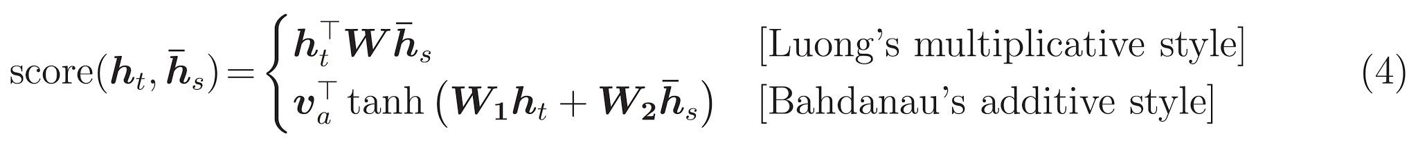
本文使用预定义的layers.Attention 实现Luong-style attention。
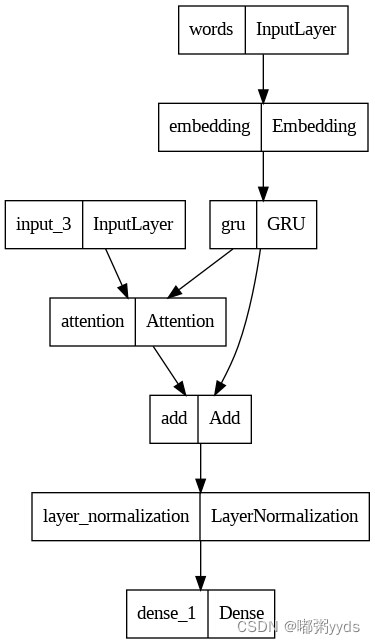
8.2.2 解码器步骤
解码器的工作是为下一个输出token生成预测。
- 解码器作为批处理接收当前单词标记。
- 它将单词标记嵌入到
ATTENTION_DIM维度。 - GRU层跟踪词嵌入,并返回GRU输出和状态。
- Bahdanau-style attention通过使用GRU输出作为查询来关注编码器的输出功能。
- attention输出和GRU输出被添加(跳过连接),并在归一化层中归一化。
- 它根据GRU输出为下一个令牌生成logit预测。
我们可以在Keras FunctionAPI中定义所有步骤,但请注意,这里我们实例化了具有可训练参数的层,以便我们在推理阶段重用层和权重。
word_input = Input(shape=(MAX_CAPTION_LEN), name="words")
embed_x = Embedding(VOCAB_SIZE, ATTENTION_DIM)(word_input)

decoder_gru = GRU(
    ATTENTION_DIM,
    return_sequences=True,
    return_state=True,
)
gru_output, gru_state = decoder_gru(embed_x)

decoder_atention = Attention()
context_vector = decoder_atention([gru_output, encoder_output])

addition = Add()([gru_output, context_vector])

layer_norm = LayerNormalization(axis=-1)
layer_norm_out = layer_norm(addition)

decoder_output_dense = Dense(VOCAB_SIZE)
decoder_output = decoder_output_dense(layer_norm_out)
decoder = tf.keras.Model(
    inputs=[word_input, encoder_output], outputs=decoder_output
)
tf.keras.utils.plot_model(decoder)  # Google Colab已经自带了pydot和graphviz,如果是在其他环境运行则需安装这两个库
decoder.summary()
Model: "model_1"
_______________________________________________________________________________________________
 Layer (type)                   Output Shape         Param #     Connected to
===============================================================================================
 words (InputLayer)             [(None, 64)]         0           []

 embedding (Embedding)          (None, 64, 512)      10240000    ['words[0][0]']

 gru (GRU)                      [(None, 64, 512),    1575936     ['embedding[1][0]']
                                 (None, 512)]

 input_3 (InputLayer)           [(None, 64, 512)]    0           []

 attention (Attention)          (None, 64, 512)      0           ['gru[1][0]',
                                                                  'input_3[0][0]']

 add (Add)                      (None, 64, 512)      0           ['gru[1][0]',
                                                                  'attention[1][0]']

 layer_normalization (LayerNorm  (None, 64, 512)     1024        ['add[1][0]']
 alization)

 dense_1 (Dense)                (None, 64, 20000)    10260000    ['layer_normalization[1][0]']

===============================================================================================
Total params: 22,076,960
Trainable params: 22,076,960
Non-trainable params: 0
_______________________________________________________________________________________________
9 训练模型
现在我们定义了编码器和解码器。让我们将它们组合成一个图像模型进行训练。
它有两个输入(image_input和word_input,以及一个输出(decoder_output)。此定义应与数据集管道的定义相对应。
image_caption_train_model = tf.keras.Model(
    inputs=[image_input, word_input], outputs=decoder_output
)
10 损失函数
损失函数是一个简单的交叉熵,但我们在计算它时需要去掉填充(0)。所以这里我们提取句子的长度(非0部分),并仅计算有效句子部分的损失平均值。
loss_object = tf.keras.losses.SparseCategoricalCrossentropy(
    from_logits=True, reduction="none"
)


def loss_function(real, pred):
    loss_ = loss_object(real, pred)

    mask = tf.math.logical_not(tf.math.equal(real, 0))
    mask = tf.cast(mask, dtype=tf.int32)
    sentence_len = tf.reduce_sum(mask)
    loss_ = loss_[:sentence_len]  # 根据句子的长度对损失值进行截断操作,避免填充部分对损失的影响。

    return tf.reduce_mean(loss_, 1)

image_caption_train_model.compile(
    optimizer="adam",
    loss=loss_function,
)
11 循环训练
现在我们可以使用标准的model.fitAPI训练模型。
使用Google Colab里的NVIDIA T4 GPU训练1个epoch大约需要15分钟。本文仅训练了3个epoch,若读者有兴趣可增加epoch。
%%time
history = image_caption_train_model.fit(batched_ds, epochs=3)
"""输出如下:
Epoch 1/3
323/323 [==============================] - 1017s 3s/step - loss: 0.8762
Epoch 2/3
323/323 [==============================] - 987s 3s/step - loss: 0.4971
Epoch 3/3
323/323 [==============================] - 978s 3s/step - loss: 0.4279
CPU times: user 41min 58s, sys: 4min 38s, total: 46min 36s
Wall time: 50min 37s
"""
在训练阶段,模型会根据输入数据和真实标签进行训练,逐步优化权重和损失函数。但在推理阶段,我们希望能够逐步生成文本描述,而不是一次性生成完整的描述。为了实现这一目标,我们需要在生成每个单词时,将之前的状态传递给解码器,并用于生成下一个单词。
所以我们需要在描述生成期间跟踪GRU状态,并在下一个时间步骤将预测词作为输入传递给解码器。
因此,下面这段代码中创建的预测模型包含了输入层word_input、gru_state_input和encoder_output,以及输出层decoder_output和gru_state。通过将先前的状态作为输入传递给解码器,并将更新后的状态作为输出,可以在生成文本描述时保持状态的连续性,从而逐步生成合理的文本序列。
gru_state_input = Input(shape=(ATTENTION_DIM), name="gru_state_input")

# 复用经过训练的GRU,但更新它以便它可以接收状态。
gru_output, gru_state = decoder_gru(embed_x, initial_state=gru_state_input)

# 也复用其他层
context_vector = decoder_atention([gru_output, encoder_output])
addition_output = Add()([gru_output, context_vector])
layer_norm_output = layer_norm(addition_output)

decoder_output = decoder_output_dense(layer_norm_output)

# 定义具有状态输入和输出的预测模型
decoder_pred_model = tf.keras.Model(
    inputs=[word_input, gru_state_input, encoder_output],
    outputs=[decoder_output, gru_state],
)
- 将GRU状态初始化为零向量。
- 预处理输入图像,将其传递给编码器,并提取图像特征。
- 设置
<start>的单词标记以开始字幕。 - 在for循环中,我们
- 将单词标记(
dec_input)、GRU状态(gru_state)和图像特征(features)传递到预测解码器并获得预测(predictions),以及更新的GRU状态。 - 从logits中选择Top-K单词,并概率地选择一个单词,这样我们就可以避免在VOCAB_SIZE大小的向量上计算softmax。
- 当模型预测
<end>标记时停止预测。 - 将输入的单词标记替换为预测的单词标记以进行下一步。
- 将单词标记(
# 定义一个句子最小长度的阈值
MINIMUM_SENTENCE_LENGTH = 5


## 使用训练模型的概率预测
def predict_caption(filename):
    # 初始化解码器状态
    gru_state = tf.zeros((1, ATTENTION_DIM))

    img = tf.image.decode_jpeg(tf.io.read_file(filename), channels=IMG_CHANNELS)
    img = tf.image.resize(img, (IMG_HEIGHT, IMG_WIDTH))
    img = img / 255

    features = encoder(tf.expand_dims(img, axis=0))
    dec_input = tf.expand_dims([word_to_index("<start>")], 1)
    result = []
    for i in range(MAX_CAPTION_LEN):
        predictions, gru_state = decoder_pred_model(
            [dec_input, gru_state, features]
        )

        # 从预测给出的日志分布中选择概率最高的前k个单词
        top_probs, top_idxs = tf.math.top_k(
            input=predictions[0][0], k=10, sorted=False
        )
        chosen_id = tf.random.categorical([top_probs], 1)[0].numpy()
        predicted_id = top_idxs.numpy()[chosen_id][0]

        result.append(tokenizer.get_vocabulary()[predicted_id])

        if predicted_id == word_to_index("<end>"):
            return img, result

        dec_input = tf.expand_dims([predicted_id], 1)

    return img, result
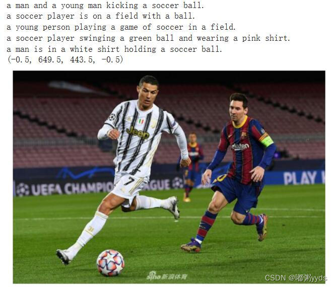
12 场景描述测试
# 待生成字幕的图片文件名
filename = "sample.png"

for i in range(5):
    image, caption = predict_caption(filename)
    print(" ".join(caption[:-1]) + ".")

img = tf.image.decode_image(tf.io.read_file(filename), channels=IMG_CHANNELS)
plt.imshow(img)


 1119
1119

 被折叠的 条评论
为什么被折叠?
被折叠的 条评论
为什么被折叠?
 到【灌水乐园】发言


