基于TensorFlow实现的自动语音识别（附项目资源）

粥粥坠腻害

已于 2023-08-15 18:14:07 修改

阅读量2.4k

点赞数 8

分类专栏：人工智能深度学习 python 文章标签：人工智能深度学习 tensorflow 语音识别 AudioLM nlp

于 2023-08-15 17:04:18 首次发布

本文链接：https://blog.csdn.net/zzp20031120/article/details/132296160

版权

python 同时被 3 个专栏收录

14 篇文章 1 订阅

订阅专栏

人工智能

13 篇文章 0 订阅

订阅专栏

深度学习

13 篇文章 0 订阅

订阅专栏

2.2.2 提取文本标注和语音文件路径，保留中文并去掉空格

开发环境

作者：嘟粥yyds
时间：2023年8月15日
集成开发工具：Jupyter Notebook 6.5.2
集成开发环境：Python 3.10.6
第三方库：tensorflow-gpu 2.10.0、librosa、matplotlib、mpl_toolkits.axes_gridl、numpy、glob、tqdm、IPython、scipy、pickle、random、os

0 概要

语音识别以语音为研究对象，它是语音信号处理的一个重要研究发现，是模型识别的一个分支，涉及到生理学、心理学、语言学、计算机科学以及信号处理等诸多领域。甚至还涉及到人的体态语言，最终目标是实现人与机器进行自然语言通信。

1 自动语音识别

1.1 简介

自动语音识别（Automatic Speech Recognition，ASR）是一项将人类说话的语音转换成文本或命令的技术。它是自然语言处理（NLP）领域的一个重要分支，旨在使计算机能够理解和处理人类语音。

ASR 技术的工作过程可以简要描述如下：

音频采集：ASR系统首先会收集来自麦克风、电话、录音等设备的声音信号，这些信号会被转换成数字形式以便计算机处理。
预处理：采集到的声音信号可能包含噪音、回声等干扰，因此需要进行预处理，以提高后续识别的准确性。常见的预处理步骤包括降噪、声学特征提取等。
特征提取：从预处理的声音信号中提取有用的特征。通常使用梅尔频率倒谱系数（MFCC）等方法来捕捉声音频谱的特征。
声学模型：声学模型是ASR系统的核心部分，它使用大量标注好的音频与文本数据来学习如何将声音特征映射到文字。传统的声学模型采用隐马尔可夫模型（HMM），而现代的方法则使用深度学习技术，如卷积神经网络（CNN）和长短时记忆网络（LSTM）来构建更准确的模型。
语言模型：除了声学模型，ASR系统还使用语言模型来提高识别的准确性。语言模型基于大量文本数据，学习语言的语法和词汇使用规律，从而帮助选择最可能的识别结果。
解码：在特征提取和模型训练后，ASR系统会对新的声音输入进行解码，找到最可能的文本结果。解码过程可能涉及到动态时间规整（DTW）等技术。
后处理：最终的识别结果可能会经过后处理步骤，以进一步优化文本的可读性和准确性，如拼写校正等。

ASR技术在很多领域有广泛的应用，包括但不限于：

语音助手和虚拟助手：比如苹果的Siri、亚马逊的Alexa和谷歌的Google助手，它们能够根据用户的语音指令提供信息、执行任务等。
电话客服：许多公司使用ASR技术来实现自动化的电话客服，让用户通过语音与计算机系统交互。
字幕生成：ASR可以将视频中的说话内容转换成文字字幕，使视频更易于理解和搜索。
医疗文档记录：在医疗领域，医生可以通过语音记录患者信息，然后ASR将其转化为文本。

然而，尽管ASR技术取得了巨大的进展，但在面对多种语音、口音、背景噪音等复杂情境时，识别的准确性仍然可能受到一定限制。随着深度学习和人工智能的发展，预计ASR技术将会不断进步并应用于更多领域。

1.2 技术原理

ASR的输入是语音片段，输出是对应的文本内容。使用深度神经网络（Deep Neural Networks， DNN）实现ASR的一般流程如下。

从原始语音到声学特征；
将声学特征输入到神经网络，输出对应的概率；
根据概率输出文本序列。

一种常用的声学特征是梅尔频率倒谱系数（Mel Frequency Cepstral Coefficents，MFCC）。

将原始语言切分为小的片段后，根据每个片段计算对应的MFCC特征，即可得到一个二维数组。

其中第一个维度为小片段的个数，原始语音越长，第一个维度也越大，第二个维度为MFCC特征的维度。得到原始语音的数值表示后，就可以使用WaveNet实现ASR。

WaveNet模型结构如下所示，主要使用了多层因果空洞卷积（Causal Dilated Convocation）和Skip Connections。

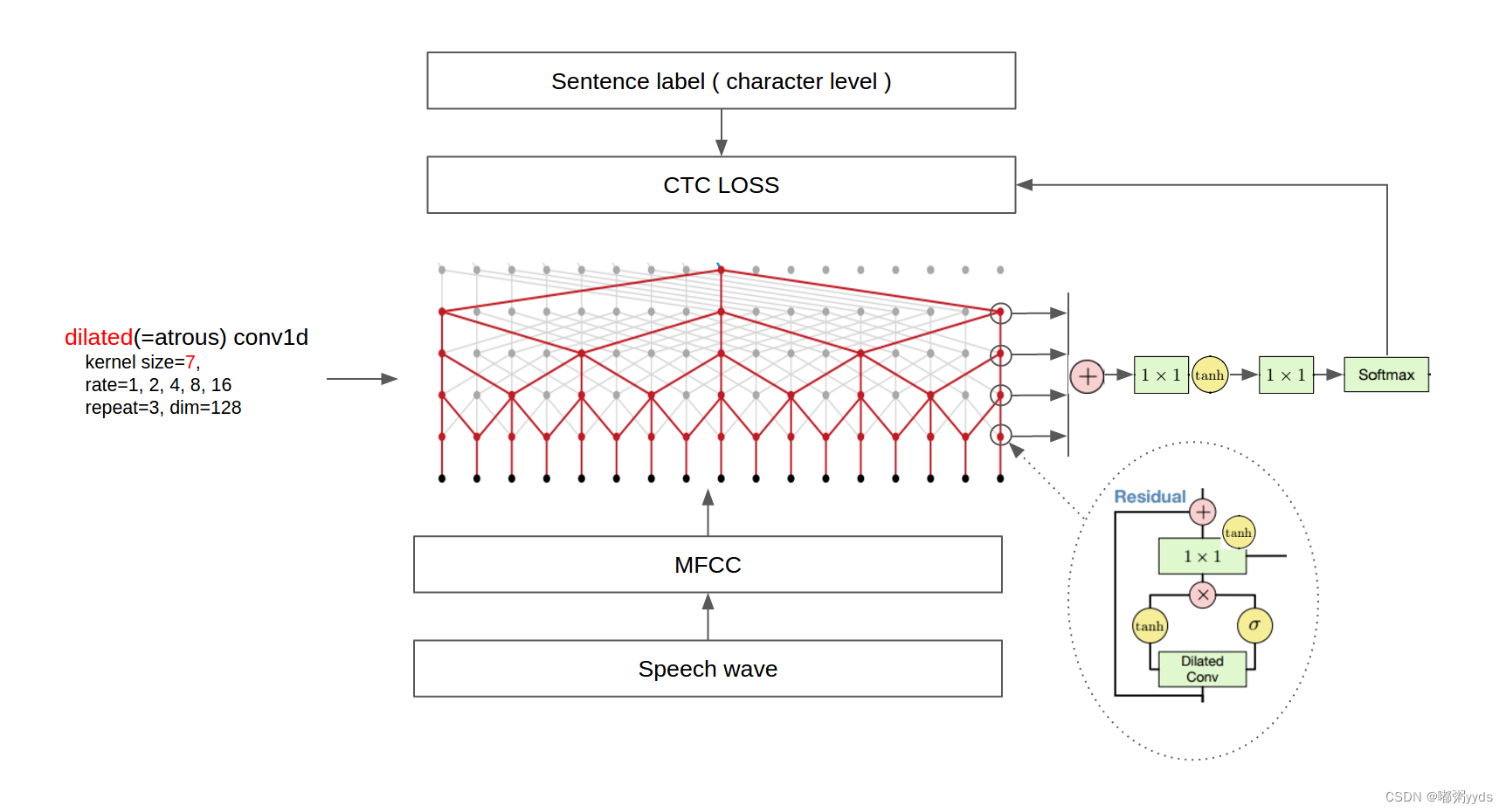
由于MFCC特征为一维序列，所以使用Conv1D进行卷积。而因果是指，卷积的输出只和当前位置之前的输入有关，即不使用未来的特征，可以理解为将卷积的位置向前偏移。

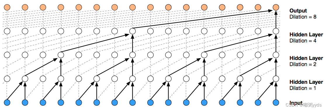
空洞是指，卷积是跳跃进行的，经过多次堆叠后可以有效地扩大感受野，从而学习到长序列之间地依赖。

最后一层卷积的特征图个数和字典大小相同，经过softmax处理后，每个小片段对应的MFCC都能得到在整个字典上的概率分布。

但小片段的个数一般要大于文本内容中字的个数，即使是同一句话，每个字的持续时间和发音轻重，字之间地停顿时间，也都有无数种可能的变化。

本文使用CTC（Connectionist temporal classification）算法来计算损失函数。

1.3 数据集

本文使用以下数据，THCHS-30，包括13388条中文语音文件以及对应的文本标注。

THCHS-30是一个很经典的中文语音数据集，包含了1万余条语音文件，大约40小时的中文语音数据，内容以文章诗句为主，全部为女声。由清华大学语言与语言技术中心（CSLT）出版的开放式中文语音数据库。原创录音于2002年由朱晓燕教授在清华大学计算机科学系智能与系统重点实验室监督下进行，原名“TCMSD”，代表“清华连续”普通话语音数据库。13年后的出版由王东博士发起，并得到了朱晓燕教授的支持。他们希望为语音识别领域的新入门的研究人员提供玩具级别的数据库。因此，该数据库对学术用户完全免费。

2 实现

2.1 导入依赖库

首先安装这个项目所特需的依赖库，若还有其他依赖库未安装，则也按相同方法安装。

pip install -i https://pypi.tuna.tsinghua.edu.cn/simple python_speech_features, librosa

# 导入其他需要的库
import numpy as np
import matplotlib.pyplot as plt
from mpl_toolkits.axes_grid1 import make_axes_locatable
%matplotlib inline
import random
import pickle
import glob
from tqdm import tqdm
import os
# 导入语音处理相关的库
from python_speech_features import mfcc
import scipy.io.wavfile as wav
import librosa
from IPython.display import Audio
# 导入所需的模块和类
import tensorflow as tf
from tensorflow.keras.layers import Input, Conv1D, Activation, Lambda, Add, Multiply, BatchNormalization
from tensorflow.keras.optimizers import SGD, Adam
from tensorflow.keras.callbacks import ModelCheckpoint, ReduceLROnPlateau, EarlyStopping
from tensorflow.keras.models import Model
from tensorflow.keras import backend as K
from tensorflow.keras.backend import ctc_batch_cost
from tensorflow.keras.utils import to_categorical, plot_model

2.2 加载数据集

2.2.1 加载文本标注路径并查看

# 使用glob匹配所有以.trn为扩展名的文件路径
text_paths = glob.glob('data/*.trn')

# 获取匹配到的文件总数
total = len(text_paths)

# 打印总文件数
print(total)


# 使用with语句打开第一个匹配到的文件
with open(text_paths[0], 'r', encoding='utf8') as fr:
    # 读取文件中的所有行并存储在lines列表中
    lines = fr.readlines()
    
    # 打印读取的行
    print(lines)

13388
['绿 是 阳春 烟 景 大块 文章 的 底色 四月 的 林 峦 更是 绿 得 鲜活 秀媚 诗意 盎然\n', 'lv4 shi4 yang2 chun1 yan1 jing3 da4 kuai4 wen2 zhang1 de5 di3 se4 si4 yue4 de5 lin2 luan2 geng4 shi4 lv4 de5 xian1 huo2 xiu4 mei4 shi1 yi4 ang4 ran2\n', 'l v4 sh ix4 ii iang2 ch un1 ii ian1 j ing3 d a4 k uai4 uu un2 zh ang1 d e5 d i3 s e4 s iy4 vv ve4 d e5 l in2 l uan2 g eng4 sh ix4 l v4 d e5 x ian1 h uo2 x iu4 m ei4 sh ix1 ii i4 aa ang4 r an2\n']

2.2.2 提取文本标注和语音文件路径，保留中文并去掉空格

# 初始化空列表，用于存储处理后的文本和文件路径
texts = []
paths = []

# 遍历匹配到的文件路径
for path in text_paths:
    # 使用with语句打开文件
    with open(path, 'r', encoding='utf8') as fr:
        # 读取文件中的所有行并存储在lines列表中
        lines = fr.readlines()
        
        # 提取第一行文本并进行处理，去除换行符和空格
        line = lines[0].strip('\n').replace(' ', '')
        
        # 将处理后的文本添加到texts列表中
        texts.append(line)
        
        # 将处理后的文件路径添加到paths列表中，去除文件扩展名
        paths.append(path.rstrip('.trn'))

# 打印第一个文件路径和对应的文本内容
print(paths[0], texts[0])

data\A11_0.wav 绿是阳春烟景大块文章的底色四月的林峦更是绿得鲜活秀媚诗意盎然

2.3 音频数据的加载、处理和可视化

mfcc_dim = 13

def load_and_trim(path):
    audio, sr = librosa.load(path)
    energy = librosa.feature.rms(y=audio)
    frames = np.nonzero(energy >= np.max(energy) / 5)
    indices = librosa.core.frames_to_samples(frames)[1]
    audio = audio[indices[0]:indices[-1]] if indices.size else audio[0:0]
    
    return audio, sr

def visualize(index):
    path = paths[index]
    text = texts[index]
    print('Audio Text:', text)
    
    audio, sr = load_and_trim(path)
    plt.figure(figsize=(12, 3))
    plt.plot(np.arange(len(audio)), audio)
    plt.title('Raw Audio Signal')
    plt.xlabel('Time')
    plt.ylabel('Audio Amplitude')
    plt.show()
    
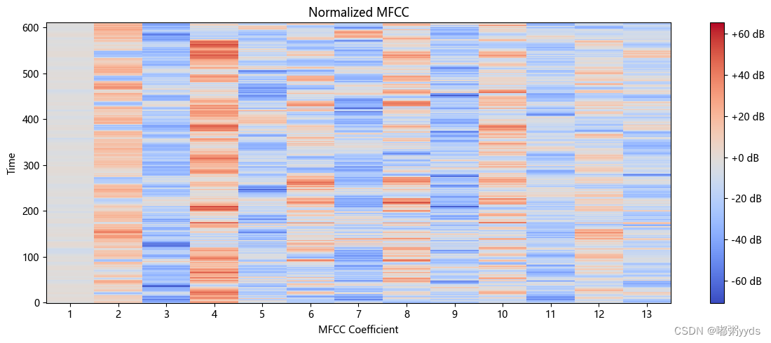
    feature = mfcc(audio, sr, numcep=mfcc_dim, nfft=551)
    print('Shape of MFCC:', feature.shape)
    
    # Plot MFCC spectrogram with coordinates
    plt.figure(figsize=(12, 5))
    librosa.display.specshow(feature, sr=sr)

    plt.title('Normalized MFCC')
    plt.ylabel('Time')
    plt.xlabel('MFCC Coefficient')
    plt.colorbar(format='%+2.0f dB')
    # Manually set x-axis tick labels for MFCC coefficients
    num_coefficients = feature.shape[0]
    plt.xticks(np.arange(0, 13), np.arange(1, 13 + 1))

    # Manually set y-axis tick labels for time
    num_frames = feature.shape[0]
    print(num_frames)
    time_in_seconds = librosa.frames_to_time(np.arange(0, num_frames, 100), sr=sr)
    time_labels = [t for t in time_in_seconds]
    plt.yticks(np.arange(0, num_frames, 100))

    plt.tight_layout()
    plt.show()

    
    return path

Audio(visualize(0))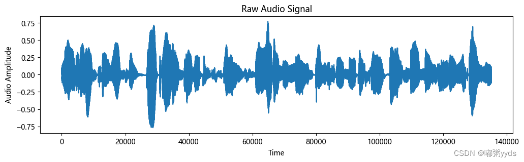

提取音频数据的MFCC特征（大概需要5分钟左右的时间）

features = []

# 使用tqdm来显示循环进度
for i in tqdm(range(total)):
    # 获取当前索引的音频文件路径
    path = paths[i]
    
    # 加载和修剪音频
    audio, sr = load_and_trim(path)
    
    # 计算音频的MFCC特征并添加到features列表中
    features.append(mfcc(audio, sr, numcep=mfcc_dim, nfft=551))
    
# 打印MFCC特征的数量和第一个特征的形状
print(len(features), features[0].shape)

# 从特征列表中随机抽取100个样本
samples = random.sample(features, 100)

# 将样本堆叠成矩阵
samples = np.vstack(samples)

# 计算抽样样本的MFCC均值和标准差
mfcc_mean = np.mean(samples, axis=0)
mfcc_std = np.std(samples, axis=0)
print(mfcc_mean)
print(mfcc_std)

# 对所有特征进行标准化
features = [(feature - mfcc_mean) / (mfcc_std + 1e-14) for feature in features]

2.4 建立字典

chars = {}

# 统计所有文本中的字符出现频次
for text in texts:
    for c in text:
        chars[c] = chars.get(c, 0) + 1

# 按字符出现频次排序
chars = sorted(chars.items(), key=lambda x: x[1], reverse=True)

# 仅保留字符列表
chars = [char[0] for char in chars]

# 打印字符数量和前100个字符
print(len(chars), chars[:100])

# 创建字符到ID的映射和ID到字符的映射
char2id = {c: i for i, c in enumerate(chars)}
id2char = {i: c for i, c in enumerate(chars)}

2883 ['的', '一', '有', '人', '了', '不', '为', '在', '是', '十', '用', '我', '外', '要', '也', '而', '中', '上', '二', '国', '他', '大', '和', '文', '来', '年', '子', '这', '到', '业', '生', '越', '于', '下', '地', '个', '以', '着', '家', '时', '月', '区', '出', '后', '成', '与', '五', '日', '能', '们', '多', '又', '可', '学', '王', '员', '三', '天', '行', '山', '发', '长', '运', '等', '因', '百', '同', '儿', '四', '得', '开', '里', '说', '就', '小', '会', '过', '作', '从', '去', '军', '之', '被', '种', '内', '应', '对', '样', '全', '厂', '民', '往', '然', '育', '所', '高', '方', '将', '明', '新']

2.5 划分数据集

2.5.1 划分训练数据和测试数据

data_index = np.arange(total)
np.random.shuffle(data_index)
train_size = int(0.9 * total)
test_size = total - train_size
train_index = data_index[:train_size]
test_index = data_index[train_size:]

X_train = [features[i] for i in train_index]
Y_train = [texts[i] for i in train_index]
X_test = [features[i] for i in test_index]
Y_test = [texts[i] for i in test_index]

2.5.2 定义批量化生成函数

本文设置的 batch_size=8 需要4G显存，读者可自行修改，训练50个epoch需要8小时左右。

batch_size = 8


def batch_generator(x, y, batch_size=batch_size):
    offset = 0
    while True:
        offset += batch_size

        if offset == batch_size or offset >= len(x):
            data_index = np.arange(len(x))
            np.random.shuffle(data_index)
            x = [x[i] for i in data_index]
            y = [y[i] for i in data_index]
            offset = batch_size

        X_data = x[offset - batch_size: offset]
        Y_data = y[offset - batch_size: offset]

        X_maxlen = max([X_data[i].shape[0] for i in range(batch_size)])
        Y_maxlen = max([len(Y_data[i]) for i in range(batch_size)])

        X_batch = np.zeros([batch_size, X_maxlen, mfcc_dim])
        Y_batch = np.ones([batch_size, Y_maxlen]) * len(char2id)
        X_length = np.zeros([batch_size, 1], dtype='int32')
        Y_length = np.zeros([batch_size, 1], dtype='int32')

        for i in range(batch_size):
            X_length[i, 0] = X_data[i].shape[0]
            X_batch[i, :X_length[i, 0], :] = X_data[i]

            Y_length[i, 0] = len(Y_data[i])
            Y_batch[i, :Y_length[i, 0]] = [char2id[c] for c in Y_data[i]]

        inputs = {'X': X_batch, 'Y': Y_batch, 'X_length': X_length, 'Y_length': Y_length}
        outputs = {'ctc': np.zeros([batch_size])}

        yield (inputs, outputs)

2.6 模型定义

# 定义自定义模块类
class ResidualBlock(Model):
    def __init__(self, filters, kernel_size, dilation_rate):
        super(ResidualBlock, self).__init__()
        self.conv1 = Conv1D(filters=filters, kernel_size=kernel_size, strides=1, padding='causal', activation=None, dilation_rate=dilation_rate)
        self.batchnorm1 = BatchNormalization()
        self.activation_tanh = Activation('tanh')
        self.activation_sigmoid = Activation('sigmoid')
        self.conv2 = Conv1D(filters=filters, kernel_size=1, strides=1, padding='valid', activation=None)
        self.batchnorm2 = BatchNormalization()
        self.add = Add()

    def call(self, inputs):
        hf = self.activation_tanh(self.batchnorm1(self.conv1(inputs)))
        hg = self.activation_sigmoid(self.batchnorm1(self.conv1(inputs)))
        h0 = Multiply()([hf, hg])

        ha = self.activation_tanh(self.batchnorm2(self.conv2(h0)))
        hs = self.activation_tanh(self.batchnorm2(self.conv2(h0)))

        return self.add([ha, inputs]), hs

# 定义其他函数
def conv1d(inputs, filters, kernel_size, dilation_rate):
    return Conv1D(filters=filters, kernel_size=kernel_size, strides=1, padding='causal', activation=None, dilation_rate=dilation_rate)(inputs)

def batchnorm(inputs):
    return BatchNormalization()(inputs)

def activation(inputs, activation):
    return Activation(activation)(inputs)

# 定义超参数
epochs = 50
num_blocks = 3
filters = 128

# 输入和卷积参数
X = Input(shape=(None, mfcc_dim,), dtype='float32', name='X')
Y = Input(shape=(None,), dtype='float32', name='Y')
X_length = Input(shape=(1,), dtype='int32', name='X_length')
Y_length = Input(shape=(1,), dtype='int32', name='Y_length')

# 构建模型
h0 = activation(batchnorm(conv1d(X, filters, 1, 1)), 'tanh')
shortcut = []
for i in range(num_blocks):
    for r in [1, 2, 4, 8, 16]:
        h0, s = ResidualBlock(filters=filters, kernel_size=7, dilation_rate=r)(h0)
        shortcut.append(s)

h1 = activation(Add()(shortcut), 'relu')
h1 = activation(batchnorm(conv1d(h1, filters, 1, 1)), 'relu')
Y_pred = activation(batchnorm(conv1d(h1, len(char2id) + 1, 1, 1)), 'softmax')
sub_model = Model(inputs=X, outputs=Y_pred)

# 构建整体模型
ctc_loss = Lambda(calc_ctc_loss, output_shape=(1,), name='ctc')([Y, sub_model.output, X_length, Y_length])
model = Model(inputs=[X, Y, X_length, Y_length], outputs=ctc_loss)
optimizer = SGD(learning_rate=0.02, momentum=0.9, nesterov=True, clipnorm=5)
model.compile(loss={'ctc': lambda ctc_true, ctc_pred: ctc_pred}, optimizer=optimizer)

# 回调和训练
checkpointer = ModelCheckpoint(filepath='full_asr.h5', verbose=0)
lr_decay = ReduceLROnPlateau(monitor='loss', factor=0.2, patience=1, min_lr=0.000)
early_stopping = EarlyStopping(monitor='val_loss', patience=5, restore_best_weights=True)

# 绘制模型结构图
plot_model(model, to_file='model.png', show_shapes=True, dpi=280)

2.7 训练并可视化误差

history = model.fit(
    x=batch_generator(X_train, Y_train),
    steps_per_epoch=len(X_train) // batch_size,
    epochs=epochs,
    validation_data=batch_generator(X_test, Y_test),
    validation_steps=len(X_test) // batch_size,
    callbacks=[checkpointer, lr_decay, early_stopping])

train_loss = history.history['loss']
valid_loss = history.history['val_loss']
plt.plot(np.linspace(1, epochs, epochs), train_loss, label='train')
plt.plot(np.linspace(1, epochs, epochs), valid_loss, label='valid')
plt.legend(loc='upper right')
plt.xlabel('Epoch')
plt.ylabel('Loss')
plt.show()

sub_model.save('sub_asr.h5')

with open('dictionary.pkl', 'wb') as fw:
    pickle.dump([char2id, id2char, mfcc_mean, mfcc_std], fw)

2.8 测试模型

下面这个代码是在训练集和测试集中随机抽取样本进行测试。

from tensorflow.keras.models import load_model
import pickle

with open('dictionary.pkl', 'rb') as fr:
    [char2id, id2char, mfcc_mean, mfcc_std] = pickle.load(fr)

sub_model = load_model('sub_asr_1.h5')

def random_predict(x, y):
    index = np.random.randint(len(x))
    feature = x[index]
    text = y[index]
    
    pred = sub_model.predict(np.expand_dims(feature, axis=0))
    pred_ids = K.eval(K.ctc_decode(pred, [feature.shape[0]], greedy=False, beam_width=10, top_paths=1)[0][0])
    pred_ids = pred_ids.flatten().tolist()
    
    print('True transcription:\n-- ', text, '\n')
    # 防止音频中出现字典中不存在的字，返回空格代替
    print('Predicted transcription:\n--  ' + ''.join([id2char.get(i, ' ') for i in pred_ids]), '\n')


random_predict(X_train, Y_train)
random_predict(X_test, Y_test)

WARNING:tensorflow:No training configuration found in the save file, so the model was *not* compiled. Compile it manually.
1/1 [==============================] - 2s 2s/step
True transcription:
--  当我病愈去医院看望您时您这个年长者却躺在病床上紧紧拉着我的手殷殷嘱我保重 

Predicted transcription:
--  当我病愈去医院看望您时您这个年长者却躺在病床上紧拉着我的手殷嘱我保重                                                                                                                                                                                                                                                                                                                                                                                                                                                                                                                                                                                                                                                                                                                                                                                      

1/1 [==============================] - 2s 2s/step
True transcription:
--  目前内蒙古拥有蒙医院二十七所中蒙医院十九所中蒙医研究所七处 

Predicted transcription:
--  目前内蒙古拥有蒙医院二十七所中蒙医院十九所中蒙医研究所七处

下面这个代码为获取本地电脑麦克风权限，记录5秒并将数据保存到本地，再用模型预测。需要提醒的是，在录音时要确保没有噪音且说话时是标准的普通话。

import pyaudio
import wave

def record_audio(output_wav_path, duration=5, sample_rate=44100, chunk_size=1024):
    audio = pyaudio.PyAudio()

    # 打开麦克风
    stream = audio.open(format=pyaudio.paInt16,
                        channels=1,
                        rate=sample_rate,
                        input=True,
                        frames_per_buffer=chunk_size)

    print("Recording...")

    frames = []

    # 监听并录制音频
    for _ in range(0, int(sample_rate / chunk_size * duration)):
        data = stream.read(chunk_size)
        frames.append(data)

    print("Recording finished.")

    # 关闭麦克风
    stream.stop_stream()
    stream.close()
    audio.terminate()

    # 保存录制的音频为 WAV 文件
    with wave.open(output_wav_path, 'wb') as wf:
        wf.setnchannels(1)
        wf.setsampwidth(audio.get_sample_size(pyaudio.paInt16))
        wf.setframerate(sample_rate)
        wf.writeframes(b''.join(frames))

        
output_wav_path = "recorded_audio.wav"
record_audio(output_wav_path, duration=5)

def single_predict(audio_path):
    # 加载和修剪音频
    audio, sr = load_and_trim(audio_path)
    
    # 计算音频的MFCC特征
    feature = mfcc(audio, sr, numcep=mfcc_dim, nfft=551)
    
    feature = (feature - mfcc_mean) / (mfcc_std + 1e-14)
    
    pred = sub_model.predict(np.expand_dims(feature, axis=0))
    pred_ids = K.eval(K.ctc_decode(pred, [feature.shape[0]], greedy=False, beam_width=10, top_paths=1)[0][0])
    pred_ids = pred_ids.flatten().tolist()
    
    print('Predicted transcription:\n--  ' + ''.join([id2char.get(i, ' ') for i in pred_ids]), '\n')

# Specify the path to your MP3 audio file
audio_path = "recorded_audio.wav"

single_predict(audio_path)

3 项目地址

项目资源地址如下：GitHub - 0911duzhou/Automatic-speech-recognition

若无法访问Github，也可在博主的主页资源里下载。

粥粥坠腻害

关注

8
点赞
踩
42

收藏

觉得还不错? 一键收藏
2
评论
基于TensorFlow实现的自动语音识别（附项目资源）

自动语音识别是一项将人类说话的语音转换成文本或命令的技术。它是自然语言处理（NLP）领域的一个重要分支，旨在使计算机能够理解和处理人类语音。本文使用TensorFlow2.x框架详细的讲解了如何进行数据处理和模型搭建，完整的刨析并实现了一个自动语音识别系统的开发流程。
复制链接

扫一扫