


Convolution is probably the most important concept in deep learning right now. It was convolution and convolutional nets that catapulted deep learning to the forefront of almost any machine learning task there is. But what makes convolution so powerful? How does it work? In this blog post I will explain convolution and relate it to other concepts that will help you to understand convolution thoroughly.
There are already some blog post regarding convolution in deep learning, but I found all of them highly confusing with unnecessary mathematical details that do not further the understanding in any meaningful way. This blog post will also have many mathematical details, but I will approach them from a conceptual point of view where I represent the underlying mathematics with images everybody should be able to understand. The first part of this blog post is aimed at anybody who wants to understand the general concept of convolution and convolutional nets in deep learning. The second part of this blog post includes advanced concepts and is aimed to further and enhance the understanding of convolution for deep learning researchers and specialists.
What is convolution?
This whole blog post will build up to answer exactly this question, but it may be very helpful to first understand in which direction this is going, so what is convolution in rough terms?
You can imagine convolution as the mixing of information. Imagine two buckets full of information which are poured into one single bucket and then mixed according to a specific rule. Each bucket of information has its own recipe, which describes how the information in one bucket mixes with the other. So convolution is an orderly procedure where two sources of information are intertwined.
Convolution can also be described mathematically, in fact, it is a mathematical operation like addition, multiplication or a derivative, and while this operation is complex in itself, it can be very useful to simplify even more complex equations. Convolutions are heavily used in physics and engineering to simplify such complex equations and in the second part — after a short mathematical development of convolution — we will relate and integrate ideas between these fields of science and deep learning to gain a deeper understanding of convolution. But for now we will look at convolution from a practical perspective.
How do we apply convolution to images?
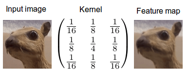
When we apply convolution to images, we apply it in two dimensions — that is the width and height of the image. We mix two buckets of information: The first bucket is the input image, which has a total of three matrices of pixels — one matrix each for the red, blue and green color channels; a pixel consists of an integer value between 0 and 255 in each color channel. The second bucket is the convolution kernel, a single matrix of floating point numbers where the pattern and the size of the numbers can be thought of as a recipe for how to intertwine the input image with the kernel in the convolution operation. The output of the kernel is the altered image which is often called a feature map in deep learning. There will be one feature map for every color channel.
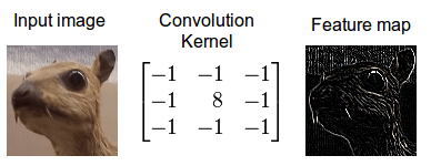 Convolution of an image with an edge detector convolution kernel. Sources:
1
2
Convolution of an image with an edge detector convolution kernel. Sources:
1
2
We now perform the actual intertwining of these two pieces of information through convolution. One way to apply convolution is to take an image patch from the input image of the size of the kernel — here we have a 100×100 image, and a 3×3 kernel, so we would take 3×3 patches — and then do an element wise multiplication with the image patch and convolution kernel. The sum of this multiplication then results in one pixel of the feature map. After one pixel of the feature map has been computed, the center of the image patch extractor slides one pixel into another direction, and repeats this computation. The computation ends when all pixels of the feature map have been computed this way. This procedure is illustrated for one image patch in the following gif.
 Convolution operation for one pixel of the resulting feature map: One image patch (red) of the original image (RAM) is multiplied by the kernel, and its sum is written to the feature map pixel (Buffer RAM).
Gif by
Glen Williamson who runs a
website that features many technical gifs.
Convolution operation for one pixel of the resulting feature map: One image patch (red) of the original image (RAM) is multiplied by the kernel, and its sum is written to the feature map pixel (Buffer RAM).
Gif by
Glen Williamson who runs a
website that features many technical gifs.
As you can see there is also a normalization procedure where the output value is normalized by the size of the kernel (9); this is to ensure that the total intensity of the picture and the feature map stays the same.
Why is convolution of images useful in machine learning?
There can be a lot of distracting information in images that is not relevant to what we are trying to achieve. A good example of this is a project I did together with Jannek Thomas in the Burda Bootcamp. The Burda Bootcamp is a rapid prototyping lab where students work in a hackathon-style environment to create technologically risky products in very short intervals. Together with my 9 colleagues, we created 11 products in 2 months. In one project I wanted to build a fashion image search with deep autoencoders: You upload an image of a fashion item and the autoencoder should find images that contain clothes with similar style.
Now if you want to differentiate between styles of clothes, the colors of the clothes will not be that useful for doing that; also minute details like emblems of the brand will be rather unimportant. What is most important is probably the shape of the clothes. Generally, the shape of a blouse is very different from the shape of a shirt, jacket, or trouser. So if we could filter the unnecessary information out of images then our algorithm will not be distracted by the unnecessary details like color and branded emblems. We can achieve this easily by convoluting images with kernels.
My colleague Jannek Thomas preprocessed the data and applied a Sobel edge detector (similar to the kernel above) to filter everything out of the image except the outlines of the shape of an object — this is why the application of convolution is often called filtering, and the kernels are often called filters (a more exact definition of this filtering processes will follow below). The resulting feature map from the edge detector kernel will be very helpful if you want to differentiate between different types of clothes, because only relevant shape information remains.
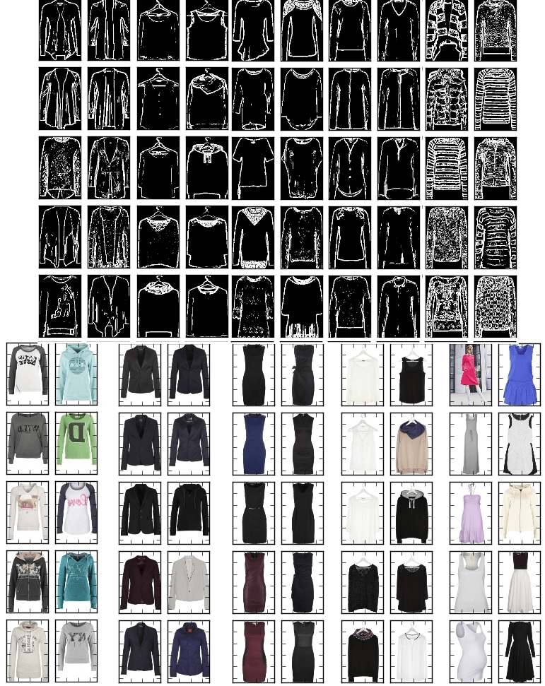 Sobel filtered inputs to and results from the trained autoencoder: The top-left image is the search query and the other images are the results which have an autoencoder code that is most similar to the search query as measured by cosine similarity. You see that the autoencoder really just looks at the shape of the search query and not its color. However, you can also see that this procedure does not work well for images of people wearing clothes (5th column) and that it is sensitive to the shapes of clothes hangers (4th column).
We can take this a step further: There are dozens of different kernels which produce many different feature maps, e.g. which sharpen the image (more details), or which blur the image (less details), and each feature map may help our algorithm to do better on its task (details, like 3 instead of 2 buttons on your jacket might be important).
Using this kind of procedure — taking inputs, transforming inputs and feeding the transformed inputs to an algorithm — is called feature engineering. Feature engineering is very difficult, and there are little resources which help you to learn this skill. In consequence, there are very few people which can apply feature engineering skillfully to a wide range of tasks. Feature engineering is — hands down — the most important skill to score well in Kaggle competitions. Feature engineering is so difficult because for each type of data and each type of problem, different features do well: Knowledge of feature engineering for image tasks will be quite useless for time series data; and even if we have two similar image tasks, it will not be easy to engineer good features because the objects in the images also determine what will work and what will not. It takes a lot of experience to get all of this right.
So feature engineering is very difficult and you have to start from scratch for each new task in order to do well. But when we look at images, might it be possible to automatically find the kernels which are most suitable for a task?
Enter convolutional nets
Convolutional nets do exactly this. Instead of having fixed numbers in our kernel, we assign parameters to these kernels which will be trained on the data. As we train our convolutional net, the kernel will get better and better at filtering a given image (or a given feature map) for relevant information. This process is automatic and is called feature learning. Feature learning automatically generalizes to each new task: We just need to simply train our network to find new filters which are relevant for the new task. This is what makes convolutional nets so powerful — no difficulties with feature engineering!
Usually we do not learn a single kernel in convolutional nets, instead we learn a hierarchy of multiple kernels at the same time. For example a 32x16x16 kernel applied to a 256×256 image would produce 32 feature maps of size 241×241 (this is the standard size, the size may vary from implementation to implementation; 
Part II: Advanced concepts
We now have a very good intuition of what convolution is, and what is going on in convolutional nets, and why convolutional nets are so powerful. But we can dig deeper to understand what is really going on within a convolution operation. In doing so, we will see that the original interpretation of computing a convolution is rather cumbersome and we can develop more sophisticated interpretations which will help us to think about convolutions much more broadly so that we can apply them on many different data. To achieve this deeper understanding the first step is to understand the convolution theorem.
The convolution theorem
To develop the concept of convolution further, we make use of the convolution theorem, which relates convolution in the time/space domain — where convolution features an unwieldy integral or sum — to a mere element wise multiplication in the frequency/Fourier domain. This theorem is very powerful and is widely applied in many sciences. The convolution theorem is also one of the reasons why the fast Fourier transform (FFT) algorithm is thought by some to be one of the most important algorithms of the 20th century.
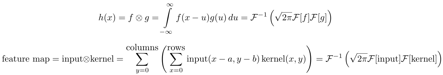
The first equation is the one dimensional continuous convolution theorem of two general continuous functions; the second equation is the 2D discrete convolution theorem for discrete image data. Here 


To get a better understanding what happens in the convolution theorem we will now look at the interpretation of Fourier transforms with respect to digital image processing.
Fast Fourier transforms
The fast Fourier transform is an algorithm that transforms data from the space/time domain into the frequency or Fourier domain. The Fourier transform describes the original function in a sum of wave-like cosine and sine terms. It is important to note, that the Fourier transform is generally complex valued, which means that a real value is transformed into a complex value with a real and imaginary part. Usually the imaginary part is only important for certain operations and to transform the frequencies back into the space/time domain and will be largely ignored in this blog post. Below you can see a visualization how a signal (a function of information often with a time parameter, often periodic) is transformed by a Fourier transform.
 Transformation of the time domain (red) into the frequency domain (blue).
Source
Transformation of the time domain (red) into the frequency domain (blue).
Source
You may be unaware of this, but it might well be that you see Fourier transformed values on a daily basis: If the red signal is a song then the blue values might be the equalizer bars displayed by your mp3 player.
The Fourier domain for images
 Images by
Fisher & Koryllos (1998).
Bob Fisher also runs an excellent
website about
Fourier transforms and image processing in general.
Images by
Fisher & Koryllos (1998).
Bob Fisher also runs an excellent
website about
Fourier transforms and image processing in general.
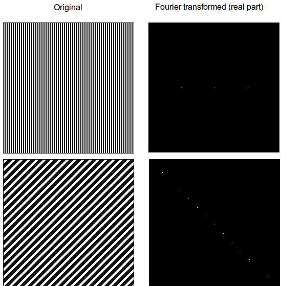
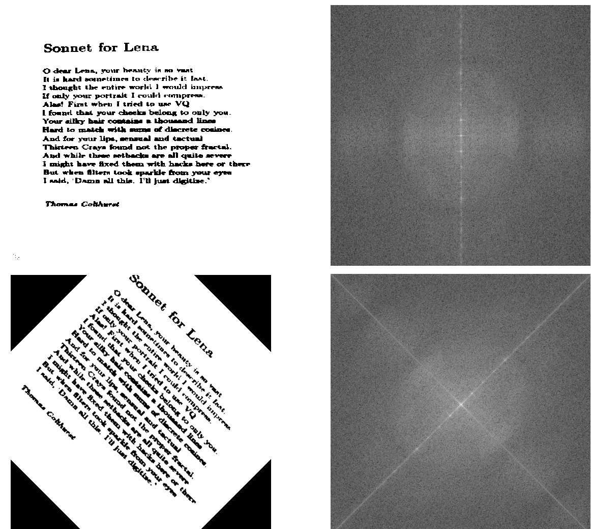
How can we imagine frequencies for images? Imagine a piece of paper with one of the two patterns from above on it. Now imagine a wave traveling from one edge of the paper to the other where the wave pierces through the paper at each stripe of a certain color and hovers over the other. Such waves pierce the black and white parts in specific intervals, for example, every two pixels — this represents the frequency. In the Fourier transform lower frequencies are closer to the center and higher frequencies are at the edges (the maximum frequency for an image is at the very edge). The location of Fourier transform values with high intensity (white in the images) are ordered according to the direction of the greatest change in intensity in the original image. This is very apparent from the next image and its log Fourier transforms (applying the log to the real values decreases the differences in pixel intensity in the image — we see information more easily this way).
 Images by
Fisher & Koryllos (1998).
Source
Images by
Fisher & Koryllos (1998).
Source
We immediately see that a Fourier transform contains a lot of information about the orientation of an object in an image. If an object is turned by, say, 37% degrees, it is difficult to tell that from the original pixel information, but very clear from the Fourier transformed values.
This is an important insight: Due to the convolution theorem, we can imagine that convolutional nets operate on images in the Fourier domain and from the images above we now know that images in that domain contain a lot of information about orientation. Thus convolutional nets should be better than traditional algorithms when it comes to rotated images and this is indeed the case (although convolutional nets are still very bad at this when we compare them to human vision).
Frequency filtering and convolution
The reason why the convolution operation is often described as a filtering operation, and why convolution kernels are often named filters will be apparent from the next example, which is very close to convolution.
 Images by
Fisher & Koryllos (1998).
Source
Images by
Fisher & Koryllos (1998).
Source
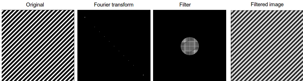
If we transform the original image with a Fourier transform and then multiply it by a circle padded by zeros (zeros=black) in the Fourier domain, we filter out all high frequency values (they will be set to zero, due to the zero padded values). Note that the filtered image still has the same striped pattern, but its quality is much worse now — this is how jpeg compression works (although a different but similar transform is used), we transform the image, keep only certain frequencies and transform back to the spatial image domain; the compression ratio would be the size of the black area to the size of the circle in this example.
If we now imagine that the circle is a convolution kernel, then we have fully fledged convolution — just as in convolutional nets. There are still many tricks to speed up and stabilize the computation of convolutions with Fourier transforms, but this is the basic principle how it is done.
Now that we have established the meaning of the convolution theorem and Fourier transforms, we can now apply this understanding to different fields in science and enhance our interpretation of convolution in deep learning.
Insights from fluid mechanics
Fluid mechanics concerns itself with the creation of differential equation models for flows of fluids like air and water (air flows around an airplane; water flows around suspended parts of a bridge). Fourier transforms not only simplify convolution, but also differentiation, and this is why Fourier transforms are widely used in the field of fluid mechanics, or any field with differential equations for that matter. Sometimes the only way to find an analytic solution to a fluid flow problem is to simplify a partial differential equation with a Fourier transform. In this process we can sometimes rewrite the solution of such a partial differential equation in terms of a convolution of two functions which then allows for very easy interpretation of the solution. This is the case for the diffusion equation in one dimension, and for some two dimensional diffusion processes for functions in cylindrical or spherical polar coordinates.
Diffusion
You can mix two fluids (milk and coffee) by moving the fluid with an outside force (mixing with a spoon) — this is called convection and is usually very fast. But you could also wait and the two fluids would mix themselves on their own (if it is chemically possible) — this is called diffusion and is usually a very slow when compared to convection.
Imagine an aquarium that is split into two by a thin, removable barrier where one side of the aquarium is filled with salt water, and the other side with fresh water. If you now remove the thin barrier carefully, the two fluids will mix together until the whole aquarium has the same concentration of salt everywhere. This process is more “violent” the greater the difference in saltiness between the fresh water and salt water.
Now imagine you have a square aquarium with 256×256 thin barriers that separate 256×256 cubes each with different salt concentration. If you remove the barrier now, there will be little mixing between two cubes with little difference in salt concentration, but rapid mixing between two cubes with very different salt concentrations. Now imagine that the 256×256 grid is an image, the cubes are pixels, and the salt concentration is the intensity of each pixel. Instead of diffusion of salt concentrations we now have diffusion of pixel information.
It turns out, this is exactly one part of the convolution for the diffusion equation solution: One part is simply the initial concentrations of a certain fluid in a certain area — or in image terms — the initial image with its initial pixel intensities. To complete the interpretation of convolution as a diffusion process we need to interpret the second part of the solution to the diffusion equation: The propagator.
Interpreting the propagator
The propagator is a probability density function, which denotes into which direction fluid particles diffuse over time. The problem here is that we do not have a probability function in deep learning, but a convolution kernel — how can we unify these concepts?
We can apply a normalization that turns the convolution kernel into a probability density function. This is just like computing the softmax for output values in a classification tasks. Here the softmax normalization for the edge detector kernel from the first example above.
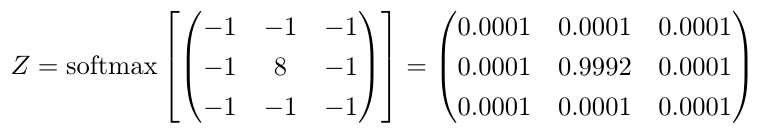 Softmax of an edge detector: To calculate the softmax normalization, we taking each value [latex background="ffffff"]{x}[/latex] of the kernel and apply [latex background="ffffff"]{e^x}[/latex]. After that we divide by the sum of all [latex background="ffffff"]{e^x}[/latex]. Please note that this technique to calculate the softmax will be fine for most convolution kernels, but for more complex data the computation is a bit different to ensure numerical stability (floating point computation is inherently unstable for very large and very small values and you have to carefully navigate around troubles in this case).
Now we have a full interpretation of convolution on images in terms of diffusion. We can imagine the operation of convolution as a two part diffusion process: Firstly, there is strong diffusion where pixel intensities change (from black to white, or from yellow to blue, etc.) and secondly, the diffusion process in an area is regulated by the probability distribution of the convolution kernel. That means that each pixel in the kernel area, diffuses into another position within the kernel according to the kernel probability density.
For the edge detector above almost all information in the surrounding area will concentrate in a single space (this is unnatural for diffusion in fluids, but this interpretation is mathematically correct). For example all pixels that are under the 0.0001 values, will very likely flow into the center pixel and accumulate there. The final concentration will be largest where the largest differences between neighboring pixels are, because here the diffusion process is most marked. In turn, the greatest differences in neighboring pixels is there, where the edges between different objects are, so this explains why the kernel above is an edge detector.
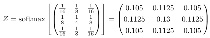
So there we have it: Convolution as diffusion of information. We can apply this interpretation directly on other kernels. Sometimes we have to apply a softmax normalization for interpretation, but generally the numbers in itself say a lot about what will happen. Take the following kernel for example. Can you now interpret what that kernel is doing? Click here to find the solution (there is a link back to this position).
Wait, there is something fishy here
How come that we have deterministic behavior if we have a convolution kernel with probabilities? We have to interpret that single particles diffuse according to the probability distribution of the kernel, according to the propagator, don’t we?
Yes, this is indeed true. However, if you take a tiny piece of fluid, say a tiny drop of water, you still have millions of water molecules in that tiny drop of water, and while a single molecule behaves stochastically according to the probability distribution of the propagator, a whole bunch of molecules have quasi deterministic behavior —this is an important interpretation from statistical mechanics and thus also for diffusion in fluid mechanics. We can interpret the probabilities of the propagator as the average distribution of information or pixel intensities; Thus our interpretation is correct from a viewpoint of fluid mechanics. However, there is also a valid stochastic interpretation for convolution.
Insights from quantum mechanics
The propagator is an important concept in quantum mechanics. In quantum mechanics a particle can be in a superposition where it has two or more properties which usually exclude themselves in our empirical world: For example, in quantum mechanics a particle can be at two places at the same time — that is a single object in two places.
However, when you measure the state of the particle — for example where the particle is right now — it will be either at one place or the other. In other terms, you destroy the superposition state by observation of the particle. The propagator then describes the probability distribution where you can expect the particle to be. So after measurement a particle might be — according to the probability distribution of the propagator — with 30% probability in place A and 70% probability in place B.
If we have entangled particles (spooky action at a distance), a few particles can hold hundreds or even millions of different states at the same time — this is the power promised by quantum computers.
So if we use this interpretation for deep learning, we can think that the pixels in an image are in a superposition state, so that in each image patch, each pixel is in 9 positions at the same time (if our kernel is 3×3). Once we apply the convolution we make a measurement and the superposition of each pixel collapses into a single position as described by the probability distribution of the convolution kernel, or in other words: For each pixel, we choose one pixel of the 9 pixels at random (with the probability of the kernel) and the resulting pixel is the average of all these pixels. For this interpretation to be true, this needs to be a true stochastic process, which means, the same image and the same kernel will generally yield different results. This interpretation does not relate one to one to convolution but it might give you ideas how to the apply convolution in stochastic ways or how to develop quantum algorithms for convolutional nets. A quantum algorithm would be able to calculate all possible combinations described by the kernel with one computation and in linear time/qubits with respect to the size of image and kernel.
Insights from probability theory
Convolution is closely related to cross-correlation. Cross-correlation is an operation which takes a small piece of information (a few seconds of a song) to filter a large piece of information (the whole song) for similarity (similar techniques are used on youtube to automatically tag videos for copyrights infringements).
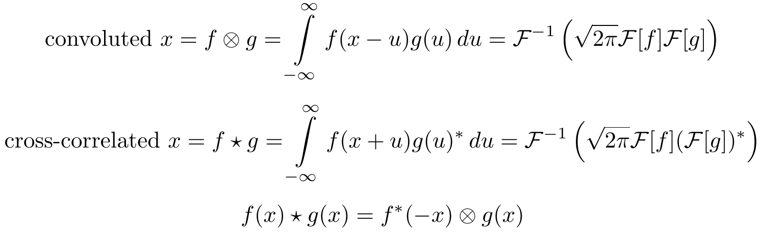 Relation between cross-correlation and convolution: Here [latex background="ffffff"]{\star}[/latex] denotes cross correlation and [latex background="ffffff"]{f^*}[/latex] denotes the complex conjugate of [latex background="ffffff"]{f}[/latex].
While cross correlation seems unwieldy, there is a trick with which we can easily relate it to convolution in deep learning: For images we can simply turn the search image upside down to perform cross-correlation through convolution. When we perform convolution of an image of a person with an upside image of a face, then the result will be an image with one or multiple bright pixels at the location where the face was matched with the person.
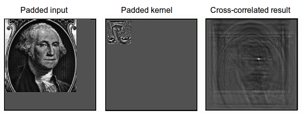 Cross-correlation via convolution: The input and kernel are padded with zeros and the kernel is rotated by 180 degrees. The white spot marks the area with the strongest pixel-wise correlation between image and kernel. Note that the output image is in the spatial domain, the inverse Fourier transform was already applied. Images taken from
Steven Smith’s excellent free
online book about digital signal processing.
Cross-correlation via convolution: The input and kernel are padded with zeros and the kernel is rotated by 180 degrees. The white spot marks the area with the strongest pixel-wise correlation between image and kernel. Note that the output image is in the spatial domain, the inverse Fourier transform was already applied. Images taken from
Steven Smith’s excellent free
online book about digital signal processing.
This example also illustrates padding with zeros to stabilize the Fourier transform and this is required in many version of Fourier transforms. There are versions which require different padding schemes: Some implementation warp the kernel around itself and require only padding for the kernel, and yet other implementations perform divide-and-conquer steps and require no padding at all. I will not expand on this; the literature on Fourier transforms is vast and there are many tricks to be learned to make it run better — especially for images.
At lower levels, convolutional nets will not perform cross correlation, because we know that they perform edge detection in the very first convolutional layers. But in later layers, where more abstract features are generated, it is possible that a convolutional net learns to perform cross-correlation by convolution. It is imaginable that the bright pixels from the cross-correlation will be redirected to units which detect faces (the Google brain project has some units in its architecture which are dedicated to faces, cats etc.; maybe cross correlation plays a role here?).
Insights from statistics
What is the difference between statistical models and machine learning models? Statistical models often concentrate on very few variables which can be easily interpreted. Statistical models are built to answer questions: Is drug A better than drug B?
Machine learning models are about predictive performance: Drug A increases successful outcomes by 17.83% with respect to drug B for people with age X, but 22.34% for people with age Y.
Machine learning models are often much more powerful for prediction than statistical models, but they are not reliable. Statistical models are important to reach accurate and reliable conclusions: Even when drug A is 17.83% better than drug B, we do not know if this might be due to chance or not; we need statistical models to determine this.
Two important statistical models for time series data are the weighted moving average and the autoregressive models which can be combined into the ARIMA model (autoregressive integrated moving average model). ARIMA models are rather weak when compared to models like long short-term recurrent neural networks, but ARIMA models are extremely robust when you have low dimensional data (1-5 dimensions). Although their interpretation is often effortful, ARIMA models are not a blackbox like deep learning algorithms and this is a great advantage if you need very reliable models.
It turns out that we can rewrite these models as convolutions and thus we can show that convolutions in deep learning can be interpreted as functions which produce local ARIMA features which are then passed to the next layer. This idea however, does not overlap fully, and so we must be cautious and see when we really can apply this idea.
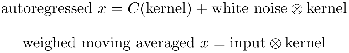
Here }")
When we pre-process data we make it often very similar to white noise: We often center it around zero and set the variance/standard deviation to one. Creating uncorrelated variables is less often used because it is computationally intensive, however, conceptually it is straight forward: We reorient the axes along the eigenvectors of the data.
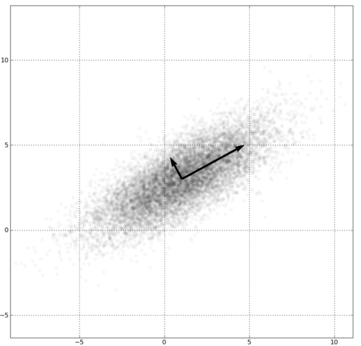 Decorrelation by reorientation along eigenvectors: The eigenvectors of this data are represented by the arrows. If we want to decorrelate the data, we reorient the axes to have the same direction as the eigenvectors. This technique is also used in PCA, where the dimensions with the least variance (shortest eigenvectors) are dropped after reorientation.
Now, if we take
The interpretation of the weighted moving average is simple: It is just standard convolution on some data (input) with a certain weight (kernel). This interpretation becomes clearer when we look at the Gaussian smoothing kernel at the end of the page. The Gaussian smoothing kernel can be interpreted as a weighted average of the pixels in each pixel’s neighborhood, or in other words, the pixels are averaged in their neighborhood (pixels “blend in”, edges are smoothed).
While a single kernel cannot create both, autoregressive and weighted moving average features, we usually have multiple kernels and in combination all these kernels might contain some features which are like a weighted moving average model and some which are like an autoregressive model.
Conclusion
In this blog post we have seen what convolution is all about and why it is so powerful in deep learning. The interpretation of image patches is easy to understand and easy to compute but it has many conceptual limitations. We developed convolutions by Fourier transforms and saw that Fourier transforms contain a lot of information about orientation of an image. With the powerful convolution theorem we then developed an interpretation of convolution as the diffusion of information across pixels. We then extended the concept of the propagator in the view of quantum mechanics to receive a stochastic interpretation of the usually deterministic process. We showed that cross-correlation is very similar to convolution and that the performance of convolutional nets may depend on the correlation between feature maps which is induced through convolution. Finally, we finished with relating convolution to autoregressive and moving average models.
Personally, I found it very interesting to work on this blog post. I felt for long time that my undergraduate studies in mathematics and statistics were wasted somehow, because they were so unpractical (even though I study applied math). But later — like an emergent property — all these thoughts linked together and practically useful understanding emerged. I think this is a great example why one should be patient and carefully study all university courses — even if they seem useless at first.
 Solution to the quiz above: The information diffuses nearly equally among all pixels; and this process will be stronger for neighboring pixels that differ more. This means that sharp edges will be smoothed out and information that is in one pixel, will diffuse and mix slightly with surrounding pixels. This kernel is known as a Gaussian blur or as Gaussian smoothing.
Continue reading. Sources:
1
2
Solution to the quiz above: The information diffuses nearly equally among all pixels; and this process will be stronger for neighboring pixels that differ more. This means that sharp edges will be smoothed out and information that is in one pixel, will diffuse and mix slightly with surrounding pixels. This kernel is known as a Gaussian blur or as Gaussian smoothing.
Continue reading. Sources:
1
2
Image source reference
R. B. Fisher, K. Koryllos, “Interactive Textbooks; Embedding Image Processing Operator Demonstrations in Text”, Int. J. of Pattern Recognition and Artificial Intelligence, Vol 12, No 8, pp 1095-1123, 1998.
-
Ivan says
-
Tim Dettmers says
That was exactly, what I wanted to achieve — thanks for your feedback!
-
-
Arun Aniyan says
This is the best post I have read which introduces convolutional NNs in an easy and understandable manner.
Looking forward to see more.-
Glad you found the blog post useful. In my next big blog post I will relate deep learning with integrative neuroscience, psychology and I will analyse in how far deep learning can be compared to the brain. I think I will be able to write everything up in the next 3-4 weeks. I also might write a smaller blog post in-between.
-
Stathis Fotiadis says
Oh that would be great to read. The intersection between ML and neuroscience is very interesting especially from a probabilistic inference and information theoretic point of view.
Grabbing the opportunity to say that this was a great article Tim.
Intuitive explanations help so much to especially on state-of-the-art things that are not yet inside the collective knowledge domain.-
Thanks!
I am also excited to write up that article. I think the intersection between deep learning and information theoretic point of view will be most important for deep learning researcher. But I will also focus on high level structure in the brain, like modules and integrated modules. Although often underestimated, I believe that a good understanding of these integrated systems will be very important to make significant progress in the deep learning.
-
-
-
-
Sergey Kuznetsov says
Tim,
Thanks a lot for your Convolution Tutorial!
It makes sense for me now after reading it.
I enjoyed reading your tutorial the same way I enjoyed taking Andrew Ng’s Machine Learning coursera course. The same way of representing complicate stuff in simple analogies.
This is the way I understand it best!Thanks a lot again! And I hope that you will write more of these great tutorials!
-
EvanZ says
Interesting post. Reminds me of a lot of the image processing I did in my grad schools. Really, it seems to me the convolution is a part of the pre-processing part of feature engineering, and not so much an inherent part of the learning algorithm itself.
-
adalyac says
tour de force Tim! gah, going to take me a while to get the intuition.
cannot intuit from the image examples the mapping between real part of fourier transform and original image. would love to be able to interactively modify the real part image (say by adding white dots or lines) and see how this alters the original image.
I’ll try reading other material and coming back to this over next few days!
other questions:
when you give formula for discrete convolution:
is kernel(x,y) constant over x,y?
what do a,b represent?-
am struggling to untuit from wave piercing paper because:
1. you say wave travelling from 1 edge of image to other; do you mean from left to right, top to bottom, or does it depend, and if so, how?
2. should I picture a wavy line or a wavy plane piercing through the paper?
3. does wave pierce through paper always when certain color and always hovers over other color, or does it pierce sometimes when black, sometimes when white? (“such waves pierce the black and white parts”)
4. how to interpret axes of real part of fourier transform of image?this post seems like a gold mine for intuiting the importance of convolutions, I can’t wait to “get it”!
-
1. Its from left to right and top to bottom and these values are multiplied with each other, so that values with high intensity only occur if both left to right and top to bottom waves have high intensities/coefficients. If you apply the log transform you will see more values than just the two dots in the one image, but these values are not visible normally because they are about about a hundred times dimmer.
2. Wavy lines one pixel wide
3. For more complex images this is not as straightforward and waves will not exactly pierce all colors (very few will do). For more complex images you can imagine the images to be a mountain landscape where each color is a peak with a certain height: Black has a height of 0 and white a height of 255 (and gray a height inbetween). If you now approximate this peak landscape by a sum of waves then each wave is represented as one pixel in the Fourier domain.
4. The image is mirrored through its diagonal and each axis represents the frequency of the waves that travel from top to bottom and left to right, respectively.
-
-
Generally, convolution is an operation of a non-constant valued function, but in the case of deep learning the kernel is a function of constant value (constant with respect to the current parameters; the constants change during training a conv net of course).
The parameters a and b often cannot be interpreted exactly and even if this is possible, things will be still unclear: In terms of cross-correlation it can be interpreted as the lag (time difference between the first signal from the second signal, e.g. one signal begins at time 4 another begins at time 6, so the value of a would be 6-4 = 2).
In terms of image convolutions one could think of the a and b as the sliding window over the image, but this interpretation is mathematically incorrect. One correct way — but not very useful way — is to think about
and
as the sum of two independent random variables
so that
which would turn the operation
into the convolution
— this is exactly how you calculate the probability density function for the sum
and
.
-
-
Thanks for a great post! A little offtop, but can you point to a good source of information about how to go about designing/tweaking ConvNet’s architectures? How did you figured it out when you started?
-
Training conv nets is more an art than an exact science. There is some information on how to train conv nets – like this comment from Sander Dieleman – but there is not much more because good nets vary from task to task and so there are no hard rules how to do it. The best way is just to learn it by trial and error.
People say that you learn best when you can look an expert over the shoulder; failing to have a mentor like that, the next best option is to learn by trial and error, e.g. do some kaggle competitions (those that already finished and playground competitions, try to get good results compared to others) and after you feel competent you should move on to ImageNet. Once you get a feel for ImageNet, again move away from it and gather more experiences from different data sets (maybe Kaggle, but not necessarily). After that, go back to ImageNet and apply everything you have learned and you should be just as good as the best.
Good luck!
-
-
Arun Krishnan says
A wonderful, wonderful post. Kudos to you! Loved the way you explained the mathematics. I have always maintained that if you can’t explain the mathematics through words/imagery, you don’t understand it! It’s obvious that you have a deep understanding of it. Loved your imagery of the wave piercing the image at specific parts while explaining the Fourier transforms.
-
That is a great compliment — thank you!
-
-
nusitocorp says
Thanks for this great post about convolutions in deep learning; with the chosen examples and the way that you developed the idea provides me with clear view of this topic, and again thanks for your reply about GPUs brands.
The areas of applications that you mentioned were very interesting, making me excited about the future applications of deep learning, especially in health informatics. Do you think that is mathematically possible and correct to convert a patient (signs and symptoms, laboratory values and images) using fast Fourier transform (or any other) to predict outcomes (death, disease, hospitalization)?-
I think applying convolutions makes only sense if you have information which is comparable, for example it might be useful to apply a convolution over the lipid profile of the laboratory values, or to apply convolution to symptoms as word embeddings. For example, you could learn symptoms with word2vec: I did this once for cooking recipes which works well (one line in the file is like this: “Recipe, Ingredient1, Ingredient2,…”), and this data is similar to medial data (symptoms=ingredients, recipe=disease) — so this might work well also! Once you obtained such embeddings, applying convolutions should yield pretty good features.
Also plotting such embeddings would yield a excellent visualization to quickly single out relevant disease for certain symptoms.
-
-
salemameen says
Hi Tim,
It took for me a long time to understand this valuable blog, thanks.-
Thanks for your feedback! What were the most difficult parts to understand for you? I think the transition from Fourier transform to fluid mechanics is a bit harsh and I will need to improve that in an update. What do you think?
-
-
sean says
I don’t really agree with your fourier transform analysis.
a) its easier to think of CNNs as banks of feature detectors cascaded together.. convolution is just sweeping a feature detector over the image. ‘the feature’ is represented by the neuron weights, and you use cosine similarity to ‘detect’ the feature and a threshold.
b) fourier transform is just a linear transformation, just a matrix multiplication, and so can be ‘folded into’ the weights – anything expressible in fourier domain is just as easily captured in original domain – its just a different set of weights. So it is just as easy to learn for the cnn or any other ML algo that takes a weighted sum of inputs.
c) as you say cross-correlation can be done by turning the image upside down[ so they are equivalent] – its just changing the orientation – so then ‘edge detection’ can be equally represented as cross correlation.The trick about CNNs is that it is cascades (ie multiple layers) of linear filters with non linearities in between, which is much harder to analyse and which allows more complicated calculations.
d) given your maths background you might want to look at this paper http://arxiv.org/pdf/1203.1513.pdf which attempts to get to grips with what a convolutional neural net is doing [I won’t claim I understand it!].-
Thank you, for your valuable comment. Although I thought about cross-correlation, it did not came to my mind that this could be the main reason why convolutional nets work. The interpretation that you give through (a) to (c) is very reasonable and this might be indeed the best way to think about it. It is difficult to prove for deep layers, but it seems like a very good fit for the first layer. I certainly will include it in an update to this post — thank you!
The paper in (d) seems like a hard nut to crack, but it seems equally valuable — I will put it on my reading list, thanks for the link!
-
-
ilzmaster says
Very nice post. I’ve enjoyed reading your wordpress in general and really like your explanations and advice.
I’m curious how you’ve used the many interpretations that you listed for the filters learned in CNNs in your experience. The 2014 ‘Visualizing and understanding convolutional networks’ article by Zeiler and Fergus visualized filters and improved their performance by tweaking their CNN’s structure to stop producing ‘bad’ filters according to their interpretation (first layer filters missing mid-frequency information, aliasing artifacts in the 2nd layer…).
From your kaggle experience or otherwise, are there cases where you’ve applied these interpretations to spot badly learned filters, and then tweaked structure/hyper-parameters to improve your performance? It sounds like with these richer interpretations, that there might be more ‘bad’ kinds of filters to look out for.
Thanks!
-
Thank you, I am happy that you found the information on my blog useful.
If you want to do well in a competition “fine tuning by inspection” might be helpful after you have done everything else, but overall time is often better spend with selecting a model (parameter tuning) and pre-processing data (The approach of Sander Dieleman’s team on the plankton Kaggle competition is a good example for this).
I find insights like the ones in the paper by Zeiler and Fergus particularly helpful for understanding why and how deep learning works, but also — and this is quite important for me — to understand how it relates to the brain: The brain uses many different kinds of processes which can be modeled quite well with convolution and understanding convolution brings us one step closer to understanding the brain. One very interesting fact is, that the brain uses spatial convolution only to compute vision and hearing, all other processes are not computed by spatial convolution (at least outside of neurons this is true); the brain uses our supercomputer, the cerebellum — which contains the majority of all neurons in the brain — for all tasks other than vision and hearing. The cerebellum was long thought to be used for movement alone, but new, clear evidence shows that is maps one-to-one to all other regions in the brain (except vision and hearing). I find it quite suspicious that vision and hearing does not use the cerebellum and I think understanding convolution might help to understand the cerebellum as well; I believe these the cerebellum and the visual system do something similar.
-
Mark says
If you are interested in the cerebellum, you may want to check out any book on motor learning and motor control. Cerebellum is a part of a system that integrates sensory input from the musculoskeletal system, vestibular apparatus and vision with “templates for action” then if everything checks out, releases signals down motor pathways to muscles. Lot’s of areas are involved. I am not clear what you mean that the cerebellum is for movement alone??
What I find interesting is the links to “The Perception of Probability” with our movement decision. According to the interpretation of those authors, these experiments challenge delta rule updating.
-
Indeed, the motor functions and effects of the cerebellum are well known, but I am rather interested how the cerebellum affects cognition. Recent evidence shows, that the cerebellum creates feedback loops with most brain regions in the cortex, for example computation from the cerebellum feeds back into the prefrontal cortex. There was a Nature study which showed that the best predictor for change in non-verbal IQ between ages 19-25 was associated with the anterior cerebellum — and this might give a hint that something important is going on in the cerebellum with respect to cognition.
What you say about the perception of probability challenging the delta rule is intriguing and I will look into that, thanks you!
-
-
-
-
Here are the links to a talk by one author of the probability of perception
class="youtube-player" height="390" src="http://www.youtube.com/embed/v5rEDe7Rwpg?version=3&rel=1&fs=1&autohide=2&showsearch=0&showinfo=1&iv_load_policy=1&wmode=transparent" frameborder="0" width="640" allowfullscreen="true" type="text/html">
Their paper goes into the model and it’s math.
Also, the same author uses finding about the cerebellum in a talk/debate the day before. In this talk, he argues against Hebbian learning models for long-term memory. He is challenged but neither side to me seems to win but you will need to decide that of course.
class="youtube-player" height="390" src="http://www.youtube.com/embed/JCDaURmKPm4?version=3&rel=1&fs=1&autohide=2&showsearch=0&showinfo=1&iv_load_policy=1&wmode=transparent" frameborder="0" width="640" allowfullscreen="true" type="text/html">
As an aside related to programming recurrent neural nets and getting rid of the complexity added by LSTM units but also solving the vanishing gradient problem then check this out:
“A Simple Way to Initialize Recurrent Networks of Rectified Linear Units” Quoc V. Le, Navdeep Jaitly, Geoffrey E. Hinton.
-
Thanks for the links!
-
-
Here is something that has parts in it which may come in handy:
GPU Accelerated Randomized Singular Value Decomposition and Its Application in Image Compression
-
Julienne LaChance says
Hi Tim,
Awesome post! I’m trying to learn about convnets on my own (from a background in Applied Math), and I really appreciate the way you make the material extremely visual and tie it into other fields. Can you recommend a good source for getting a better understanding of what feature maps really “mean”? For example, it’s sort of apparent why convnets pick out certain features from 2D images and videos, in that we can recognize features similar to the edge-detectors, facial characteristics, and so on that computer scientists used to engineer themselves. But what do they mean in general? Could I train a convolutional network on a physical system (fluid flow?) and use the feature maps to learn more about the important structures (coherent structures?) defining the dynamics of that system?
I’ll definitely be using your hardware guide too- thanks!
Best,
Julie-
Hi Julie,
these are excellent questions. However, I am afraid that I am unaware of any resource where feature maps are looked at in a general way. There are some papers that try to make sense of it all, but then again it is in terms of filters learned on images and despite some good results and visualization techniques the meaning of feature maps remains quite unclear.
What I find helpful is to look at what feature maps do in other contexts. For example in music recommendation where temporal convolution is used, the feature maps filter the data for features which make music genres distinct (certain type of instruments, tempo), and secondly, within a music genres, the feature map filter the data for features which makes songs similar and distinct (a certain type of beat, a certain bass-line, etc.).In natural language processing the feature maps can be used to learn grammar (part-of-speech tagging) and here they represent more or less grammatical rules (subject + verb + object and more complex rules for different tenses, auxiliary verbs etc.). Convolution can also be used to learn the meaning of a sequence of words and thus generate text which has similar meaning to a previous phrase, so here the feature map encapsulates the meaning of a subject-verb-object relation and produces new words which are related to the previous relation. However, after two sentences or so the meaning breaks down and the convolutional net then produces meaningless sentences (which may still be grammatically correct).
So seeing learned feature maps as “filters” or seeing them as “features” themselves is rather vague but this is the best general idea of a feature map that I am aware of.
I have heard about research groups trying to train convolutional nets to solve PDEs, but I never heard of any good results. I think this is a very difficult problem because tiny variations can lead to big changes and while neural networks should theoretically be able to model such relations it is practically quite difficult for a neural net to capture such minor details with limited data. I imagine producing enough data is a big problem here, because solving physical systems to acquire such data is quite computationally intensive on its own. I think one would be able to model simple fluid flow problems along common, simple objects or along pipes etc. quite well, but for more complex problems the solutions are probably not precise enough. I am sure there will be advances in the future as new algorithms and new neural architectures are found, but right now it does not seems to be possible or useful to use convolutional networks — or other models like recurrent neural networks — to model physical systems.
Best,
Tim-
Hi Tim,
Thanks for the reply! I’ve also encountered the research that you mentioned with regards to trying to solve PDEs using convnets, and I have to agree with you: the systems will always be too sensitive to initial and boundary conditions! However I think convnets have the potential to become a tool for experimental mathematics. If I’m getting stuck when trying to solve a system analytically, I would love to be able to train a network using known inputs and outputs, and let the feature maps hint at what is important for the solution!
Have you seen this paper?: http://arxiv.org/abs/1412.3409 (Teaching Deep Convolutional Neural Networks to Play Go)
The authors encode the boundary of the Go board as a padding layer of 0’s plus an extra channel with 1’s around the edges. It makes me wonder if one can encode other types of boundary conditions using a similar technique! You’re right about full-blown fluid dynamics problems being too computationally intensive at the moment, but it might be worthwhile to do a test-run of the network with a system that has a known analytical solution, and see what the features are.
A thousand more thanks for the fantastic blog! Keep it up!
Best,
Julie-
Hi Julie,
that’s a good idea. Letting a convolutional net learn what is important for the solution is much more realistic than learning the solution itself. That would probably also involve some hard work to make it work, but it would be much more manageable.
Thanks for the link to the paper. That is a very interesting application which I have not seen before. I think the boundary conditions can be quite tricky because the behaviour at those boundaries can be very different from system to system which is not so for Go. One thing which might work well is the new capsule approach developed by Geoff Hinton, where the position of a feature is also encoded by a position value (x,y,(z)) and almost no labels are needed to learn from the data. In fluid dynamics this would be great to model boundaries and boundary layers. However, this approach is still experimental and the results have not been published yet — but definitely something to look out for!
Best,
Tim
-
-
-
-
Hi Tim,
Awesome- thanks for the link! I’ll check it out and keep an eye out for applications.
Warm regards,
Julie-
Also, a friend of mine just shared this demo with me:
http://cs.stanford.edu/people/karpathy/convnetjs/demo/cifar10.html
…which trains a convnet live in your browser!
-
Just today I came across a link to the thesis of Tijmen Tieleman on the google+ deep learning community with some results using the capsule approach mentioned above. It works great on MNIST, but it does not seem to yield very significant results on other data sets (like the CIFAR10 data set in the browser demo). So this approach will probably also not be that breakthrough which would make deep learning feasible for dynamical systems. But the field of deep learning is moving fast, so there might be something around the next corner.
-
-
-
^ Even so, I appreciate the share! Indeed that method seems too slow for general problems, but it’s cool that Hinton could tailor the capsule structure to handle datasets like MNIST so well. What should we expect if there are no meaningful features? Would the convolutional layer just act like an identity operator, and let the work be done in the conventional NN layers?
-
If there are no meaningful feature there are two options. The first is more practical and occurs rather often if you take unusual data sets: When there are no useful features in the data, there are often still some random patterns in the data (even if those arise through chance, they are still patterns). If such patterns exist the convolutional net will still learn, but the error rate will only decrease on the data set where the network is trained on, and it will stay the same (or get worse) on the cross validation or test data set.
If you train a convolutional net on true random data (no patterns arise from the randomness), then the whole system will be driven by noise (all gradients will be noisy) and as such, the convolutional filters would add just noise to the data and pass its result on to the next layer; the same would be true for the final dense layers.
-
Thanks!
-
You are welcome, Julie. If you do some experiments with deep learning on dynamical systems please let me know, it would be interesting to see some results — thanks!
-
-
-
-
I will certainly keep you posted! Good luck with your own projects
-
Javier says
Hi Tim,
Great blog.
I sold like to know your opinion about the Nvidia Jetson TK1?
I’m considering to buy one/some of these to use in deep leaning (single or even parallelization)Thanks
-
The Jetson TK1 is great for small embedded projects. Because it uses 2-4 watts in idle and a maximum of about 11 watts under full load, you can power it with a battery and it will still last many hours.
Performance wise the Jetson TK1 is on a par with some smaller laptop GPUs (something like a GTX 260M) and this is mainly because the TK1 has a rather poor memory bandwidth. However, this will be sufficient to run trained convolutional nets with good speed for mobile applications. However, I would not try to train convolutional nets on a Jetson TK1, because (1) it is slow, and (2) the available memory will be limiting.
I would not try parallelization with them. While it may work for other applications (I have seen successful builds involving multiple Jetson TK1), this will not be possible for deep learning because the 1 Gbit/s ethernet will be much too slow (the very high latency on ethernet will kill parallelization, as does the low bandwidth of 1 Gbit/s).
Things might get more interesting with the if NVIDIA decides to build a Jetson based on the new Tegra X1. With four times the performance of the Jetson TK1, you could do serious training of small architectures for some applications which feature small data sets, but again, parallelization would not be feasible in this case.
-
-
aalll says
the fact that people can actually comprehend and understand this… bafffles me. I’m sure with a pen and paper to really write out the specifics and to process it myself, I could get a little closer, but even after all of that I’m not 100% sure I would still fully understand.
-
Thank you for the feedback. Are there some specific sections or ideas which are difficult or confusing? I would improve them when I come to revise the article.
-
-
antonio says
Very good man, finally i understand what happen inside a convolutional layers, thank you very much!!!
-
danbenyamin says
Great article, and I want to dig in more! The opening section did harken back to my grad school EE days, and as such gave me a bit of a chill when I read things not quite right. Namely:
1. You mention in a few places “Fast Fourier Transform”, where I believe all you are referring to is the Fourier Transform. The FFT algorithm isn’t really germane to your discussion.
2. In a couple of specialized fields the term “Fourier Domain” is used, but it is almost always known as frequency domain, not Fourier domain. The Laplace and Discrete Cosine transforms also refer to frequency domains.
It may be pedantic, but I think consistent terminology for such an in-depth primer is important.
Kudos again!
-
Thanks for your comment. I think correct terminology is important and I will update this post when I can find the time.
-
-
Thank you for this well informative and constructive post of deep learning. You make my life through this post.
-
Eric says
Tim,
Amazing read. I really appreciate it. If I wanted to identify six different types of garments. Would I separate out the photos into 6 folders and run six different learning algorithms on them or would I run one algorithm on all of them?
Best Regards – Eric
-
One algorithm should be better than 6. The garments are probably related in some way (they might share “parts”) and a single model and pick up on these details and correlations and make more informed classifications. Independent models would not be able to do this.
-
-
tingting says
Hi,Tim. Thanks so much for your blog. It is so great and helps me a lot. I want to ask you a question about the 2D correlation and 2D convolution. It is known that the only difference 2D correlation and 2D convolution is a 180 rotation. Then why is the 2D convolution used, but not the 2D correlation? This question puzzled me a lot. Thanks very much!
-
It is not straightforward correlation, but autocorrelation, that is correlation over a sequence for each position. This is very similar to convolution but on its own does not generate good features (filters must have features of the images in them, which are not known before we run the algorithm). However, a convolutional network learns the features, and should be able to find the same features as with convolution, but convolution should be better, because it yields useful features almost immediately.
-
Hi,Tim. Thanks so much for your reply. However I am still a little puzzled.
Suppose this is an image A and a kernel B (3*3), then we can obtain the feature map C by A*B, that is to say the value of C(1,1) equals to A(1:3,1:3)*B, (here * is a convolution operation).
However we can obtain the same value of C(1,1) by A(1:3,1:3)*rotation180(B), (here * is a correlation operation).
From this view, we can obtain the same feature map by convolution and correlation.
What is wrong of this explanation? I really cannot understand. Thanks so much! -
Ming says
“At lower levels, convolutional nets will not perform cross correlation, because we know that they perform edge detection in the very first convolutional layers”. The only difference between cross-correlation and convolution is the filter is rotated by 180 degree in convolution. Since the filters are learned, it doesn’t really matter if they are rotated or not. As long as it is compatible in the forward and backward pass, we can think of them as the same thing. Actually in Caffe, convolution is implemented as cross-correlation.
The other thing I’d like to point out is that, location where there are edges give higher response to the first few convolution layers (edge detector). This aligns with the intuition behind cross correlation between the filters and the images.-
This is very insightful — thank you!
-
-
-
-
Rabindra Nath Nandi says
Hi, Tim , this is definitely a good recipe of Convolutional Neural Network . I have a question beyond this post. Is there is any way to integrate Stacked AutoEncoder with CNN for image classification task and is this process is meaningful to increase the CNN performance ?.
-
Yes this can be done and it may improve results. But often it is just to tedious to do this. Building and running a convolutional network is often simpler and yields in the end better performance. You can find an example for stacked convolutional autoencoder results here and the same for restricted Boltzmann machines here.
-
-
Jie says
Hi,Tim. Thanks so much for your blog. It helped me a lot on understanding convolution,I am wondering if it is OK to translate this blog into Chinese so that more people could benefit from your post?
-
That would be great! Feel free to do so!
-
Thanks, I will finish the translation asap and inform you when I post it on-line.
-
-
-
Emanuele Ziglioli says
Great blog post. Indeed everything is linked together (Fourier Transforms, Quantum Mechanics, Information Theory) but I saw the link in terms of Linear Algebra/Hilbert Spaces. Convolution can perhaps be seen as an operator in Hilbert Spaces. Hilber Spaces also apply to the continuous case, where the inner product is defined as an integral.
For references see Vetterli/Prandoni’s DSP course on Coursera (Vetterli’s book is freely available). There’s also an interesting Google Talk on Quantum Information Theory by Ron Garret “The Quantum Conspiracy: What Popularizers of QM Don’t Want You to Know”


 9917
9917


 到【灌水乐园】发言


Oh boy! It’s so awesome, you’re on my feedly now
I love intuitions I’ve learned from the post – that wave thing piercing the paper is the most vivid once. I’ll have to read this a few time like a scientific paper to learn all the magic pieces, but compared to the papers it’s pleasant to read! (also I love relations between different science fields)
Thanks