Python机器学习库sklearn数据预处理，数据集构建，特征选择

最新推荐文章于 2024-07-26 15:23:07 发布

thinker_1120

最新推荐文章于 2024-07-26 15:23:07 发布

阅读量6.6k

点赞数 3

分类专栏：算法实现

本文链接：https://blog.csdn.net/cymy001/article/details/78546185

版权

算法实现专栏收录该内容

38 篇文章 9 订阅

订阅专栏

from IPython.display import Image
%matplotlib inline
# Added version check for recent scikit-learn 0.18 checks
from distutils.version import LooseVersion as Version
from sklearn import __version__ as sklearn_version

处理缺省值

import pandas as pd
from io import StringIO

csv_data = '''A,B,C,D
1.0,2.0,3.0,4.0
5.0,6.0,,8.0
10.0,11.0,12.0,'''
print(type(csv_data))
# If you are using Python 2.7, you need to convert the string to unicode:
#csv_data = unicode(csv_data)

df = pd.read_csv(StringIO(csv_data))   
#StringIO的行为与file对象非常像，但它不是磁盘上文件，而是一个内存里的“文件”，可以将操作磁盘文件那样来操作StringIO
#StringIO在内存中读写str,要想把str写入StringIO：先创建一个StringIO，然后像文件一样写入即可
df
#type(df) #pandas.core.frame.DataFrame

df.isnull().sum()  #isnull判定每个位置是否是NaN,计算每一特征中：有几个样本在该特征上存在缺失
#Output:
#A    0
#B    0
#C    1
#D    1
#dtype: int64

1.)直接删除缺省值多的样本或者特征

df.dropna()   #删存在缺省值的样本

df.dropna(axis=1)   #删存在缺省值的特征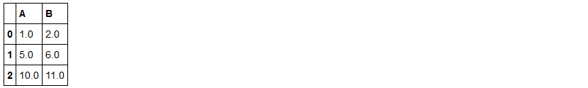

df.dropna(how='all')   #删所以特征都缺失的样本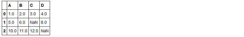

df.dropna(thresh=4)   #删特征数少于参数指定个数的样本

df.dropna(subset=['C'])   #删在指定特征处有缺失的样本

2.)重新计算缺省值

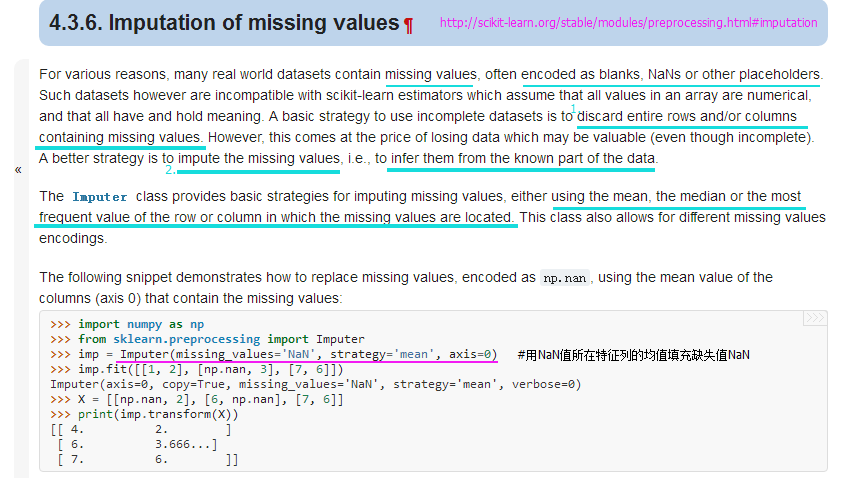
from sklearn.preprocessing import Imputer
#http://scikit-learn.org/stable/modules/generated/sklearn.preprocessing.Imputer.html#sklearn.preprocessing.Imputer
imr = Imputer(missing_values='NaN', strategy='mean', axis=0)   #用NaN所在特征列的均值填充NaN
imr = imr.fit(df)
imputed_data = imr.transform(df.values)
imputed_data
#Output:
#array([[  1. ,   2. ,   3. ,   4. ],
#       [  5. ,   6. ,   7.5,   8. ],
#       [ 10. ,  11. ,  12. ,   6. ]])

df.values
#Output:
#array([[  1.,   2.,   3.,   4.],
#       [  5.,   6.,  nan,   8.],
#       [ 10.,  11.,  12.,  nan]])

处理类别型数据

import pandas as pd
df = pd.DataFrame([['green', 'M', 10.1, 'class1'],
                   ['red', 'L', 13.5, 'class2'],
                   ['blue', 'XL', 15.3, 'class1']])
df.columns = ['color', 'size', 'price', 'classlabel']
df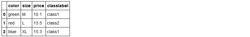

1.)序列特征映射

size_mapping = {'XL': 3,'L': 2,'M': 1}
df['size'] = df['size'].map(size_mapping)   #将size特征列的XL等字符替换成字典size_mapping映射对应的数字
df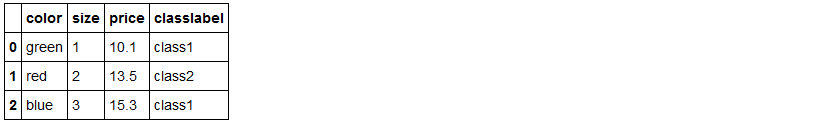

inv_size_mapping = {v: k for k, v in size_mapping.items()}   
#字典推导式，items()是将字典中键值转化成元组对，整体以列表返回
#size_mapping.items():dict_items([('XL', 3), ('L', 2), ('M', 1)])
df['size'].map(inv_size_mapping)
#Output:
#0     M
#1     L
#2    XL
#Name: size, dtype: object

2.)类别编码

import numpy as np
class_mapping = {label: idx for idx, label in enumerate(np.unique(df['classlabel']))}   
#enumerate将列表参数映射成带序号的元组对
#class_mapping作用是找出出现一个新classlabel时对应的index
class_mapping
#Output:
#{'class1': 0, 'class2': 1}

df['classlabel'] = df['classlabel'].map(class_mapping)
df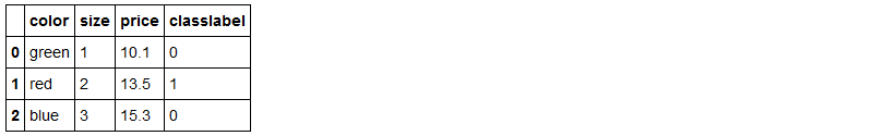

inv_class_mapping = {v: k for k, v in class_mapping.items()}
df['classlabel'] = df['classlabel'].map(inv_class_mapping)
df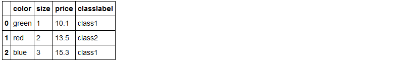

from sklearn.preprocessing import LabelEncoder
#http://scikit-learn.org/stable/modules/preprocessing_targets.html#preprocessing-targets
class_le = LabelEncoder()
y = class_le.fit_transform(df['classlabel'].values)
y
#Output:
#array([0, 1, 0], dtype=int64)

class_le.inverse_transform(y)
#Output:
#array(['class1', 'class2', 'class1'], dtype=object)

3.)对类别型的特征用one-hot编码

X = df[['color', 'size', 'price']].values
from sklearn.preprocessing import LabelEncoder
color_le = LabelEncoder()
X[:, 0] = color_le.fit_transform(X[:, 0])   #对color特征列进行顺序出现编码
X
#Output:
#array([[1, 1, 10.1],
#       [2, 2, 13.5],
#       [0, 3, 15.3]], dtype=object)

#检验color特征列编码序号原理，对应df结构看
from sklearn.preprocessing import LabelEncoder
color_le = LabelEncoder()
color_le.fit(df['color'])
#Output:
#array(['blue', 'green', 'red'], dtype=object)
color_le.classes_

from sklearn.preprocessing import OneHotEncoder
#http://scikit-learn.org/stable/modules/generated/sklearn.preprocessing.OneHotEncoder.html#sklearn.preprocessing.OneHotEncoder
ohe = OneHotEncoder(categorical_features=[0])   #categorical_features参数指定独热特征列
ohe.fit_transform(X).toarray()
#Output:
#array([[  0. ,   1. ,   0. ,   1. ,  10.1],
#       [  0. ,   0. ,   1. ,   2. ,  13.5],
#       [  1. ,   0. ,   0. ,   3. ,  15.3]])

pd.get_dummies(df[['price', 'color', 'size']])   #pandas内的独热方法get_dummies()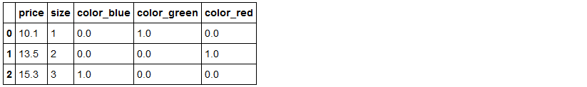

切分数据集(训练集与测试集)

df_wine = pd.read_csv('https://archive.ics.uci.edu/ml/machine-learning-databases/wine/wine.data',header=None)
df_wine.columns = ['Class label', 'Alcohol', 'Malic acid', 'Ash',
                   'Alcalinity of ash', 'Magnesium', 'Total phenols',
                   'Flavanoids', 'Nonflavanoid phenols', 'Proanthocyanins',
                   'Color intensity', 'Hue', 'OD280/OD315 of diluted wines',
                   'Proline']
print('Class labels', np.unique(df_wine['Class label']))
#df_wine.to_csv('wine.csv')
df_wine.head()
#Output:
#Class labels [1 2 3]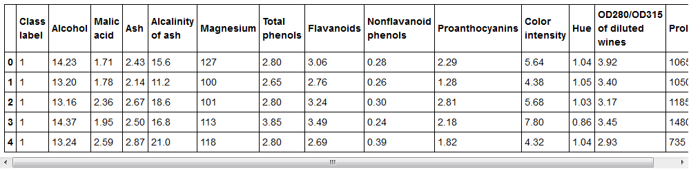

if Version(sklearn_version) < '0.18':
    from sklearn.cross_validation import train_test_split
else:
    from sklearn.model_selection import train_test_split
X, y = df_wine.iloc[:, 1:].values, df_wine.iloc[:, 0].values   #df_wine数据的第一列作为标签类别，其余列作为特征
X_train, X_test, y_train, y_test = train_test_split(X, y, test_size=0.3, random_state=0)   #全部数据的30%作为测试集

对连续值特征做幅度缩放(scaling)

from sklearn.preprocessing import MinMaxScaler
#http://scikit-learn.org/stable/modules/generated/sklearn.preprocessing.MinMaxScaler.html#sklearn.preprocessing.MinMaxScaler
#U(0,1)区间[0,1]上的均匀分布缩放，按单个特征列看
mms = MinMaxScaler()
X_train_norm = mms.fit_transform(X_train)
X_test_norm = mms.transform(X_test)
from sklearn.preprocessing import StandardScaler
#N(0,1)正态分布缩放
stdsc = StandardScaler()
X_train_std = stdsc.fit_transform(X_train)
X_test_std = stdsc.transform(X_test)

特征选择

1.) 通过L1正则化的截断型效应选择

from sklearn.linear_model import LogisticRegression
lr = LogisticRegression(penalty='l1', C=0.1)
lr.fit(X_train_std, y_train)
print('Training accuracy:', lr.score(X_train_std, y_train))
print('Test accuracy:', lr.score(X_test_std, y_test))
#Output:
#Training accuracy: 0.983870967742
#Test accuracy: 0.981481481481

lr.intercept_
#Output:
#array([-0.38380842, -0.15812178, -0.70041244])

lr.coef_
#Output:
#array([[ 0.28025703,  0.        ,  0.        , -0.02792998,  0.        ,
#         0.        ,  0.71008021,  0.        ,  0.        ,  0.        ,
#         0.        ,  0.        ,  1.23625518],
#       [-0.64387692, -0.06882766, -0.05718195,  0.        ,  0.        ,
#         0.        ,  0.        ,  0.        ,  0.        , -0.92717674,
#         0.05982319,  0.        , -0.37086571],
#       [ 0.        ,  0.06151692,  0.        ,  0.        ,  0.        ,
#         0.        , -0.63612079,  0.        ,  0.        ,  0.49812314,
#        -0.35823174, -0.57118053,  0.        ]])

import matplotlib.pyplot as plt
fig = plt.figure()
ax = plt.subplot(111)    
colors = ['blue', 'green', 'red', 'cyan', 'magenta', 'yellow', 'black',
          'pink', 'lightgreen', 'lightblue', 'gray', 'indigo', 'orange']
weights, params = [], []
for c in range(-4, 6):
    lr = LogisticRegression(penalty='l1', C=10**c, random_state=0)
    lr.fit(X_train_std, y_train)
    weights.append(lr.coef_[1])
    params.append(10**c)
weights = np.array(weights)   #10*13的数组
for column, color in zip(range(weights.shape[1]), colors):
    plt.plot(params, weights[:, column], label=df_wine.columns[column + 1], color=color)
#column+1去掉第一列label列
plt.axhline(0, color='black', linestyle='--', linewidth=1)
plt.xlim([10**(-5), 10**5])
plt.ylabel('weight coefficient')
plt.xlabel('C')
plt.xscale('log')
plt.legend(loc='upper left')
ax.legend(loc='upper center', bbox_to_anchor=(1.38, 1.03), ncol=1, fancybox=True)
# plt.savefig('./figures/l1_path.png', dpi=300)
plt.show()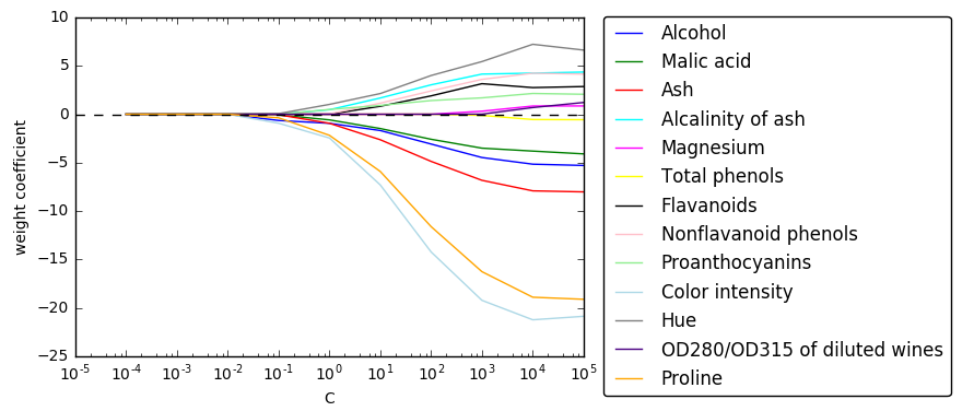

2.) 遍历子特征集选择法

from sklearn.base import clone
from itertools import combinations
import numpy as np
from sklearn.metrics import accuracy_score
#http://scikit-learn.org/stable/modules/generated/sklearn.metrics.accuracy_score.html#sklearn.metrics.accuracy_score
if Version(sklearn_version) < '0.18':
    from sklearn.cross_validation import train_test_split
else:
    from sklearn.model_selection import train_test_split

class SBS():
    def __init__(self, estimator, k_features, scoring=accuracy_score, test_size=0.25, random_state=1):
        self.scoring = scoring
        self.estimator = clone(estimator)   #构造一个具有相同参数的估计器
        #http://scikit-learn.org/stable/modules/generated/sklearn.base.clone.html#sklearn.base.clone
        self.k_features = k_features
        self.test_size = test_size
        self.random_state = random_state

    def fit(self, X, y):
        X_train, X_test, y_train, y_test = train_test_split(X, y, test_size=self.test_size, random_state=self.random_state)
        dim = X_train.shape[1]   #13
        self.indices_ = tuple(range(dim))   #(0,1,2,...,12)
        self.subsets_ = [self.indices_]
        score = self._calc_score(X_train, y_train, X_test, y_test, self.indices_)   #全特征组合得分
        self.scores_ = [score]

        while dim > self.k_features:   #至少要考虑到k_features个特征
            scores = []
            subsets = []
            for p in combinations(self.indices_, r=dim - 1):   #combinations求组合,不取全部13个特征:每次只取12个特征,11个特征...
                score = self._calc_score(X_train, y_train, X_test, y_test, p)
                scores.append(score)
                subsets.append(p)
            best = np.argmax(scores)   #argmax求分数最高的特征组合所在的索引
            self.indices_ = subsets[best]   #根据索引,取分数最高特征组合
            self.subsets_.append(self.indices_)   #同个数特征的各个组合中,得分最高的组合构成的列表
            dim -= 1
            self.scores_.append(scores[best])   #同个数特征的各个组合中,最优特征组合的得分构成的列表
        self.k_score_ = self.scores_[-1]   #每k个特征组合的最好得分,直接取scores_列表中最好加入的元素
        return self

    def transform(self, X):
        return X[:, self.indices_]

    def _calc_score(self, X_train, y_train, X_test, y_test, indices):
        self.estimator.fit(X_train[:, indices], y_train)
        y_pred = self.estimator.predict(X_test[:, indices])
        score = self.scoring(y_test, y_pred)   #用accuracy_score方法计算
        return score
#indices_是每个维度最优特征组合元组，subsets_是包含各个维度最优特征组合元组的列表，scores_是包含各个维度最优特征组合得分的列表

import matplotlib.pyplot as plt
from sklearn.neighbors import KNeighborsClassifier
knn = KNeighborsClassifier(n_neighbors=2)
# selecting features
sbs = SBS(knn, k_features=1)
sbs.fit(X_train_std, y_train)

# plotting performance of feature subsets
k_feat = [len(k) for k in sbs.subsets_]

plt.plot(k_feat, sbs.scores_, marker='o')
plt.ylim([0.7, 1.1])
plt.ylabel('Accuracy')
plt.xlabel('Number of features')
plt.grid()
plt.tight_layout()
# plt.savefig('./sbs.png', dpi=300)
plt.show()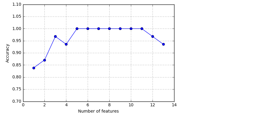

k5 = list(sbs.subsets_[8])
print(df_wine.columns[1:][k5])   #去除第一个标签列计数
#Output:
#Index(['Alcohol', 'Malic acid', 'Alcalinity of ash', 'Hue', 'Proline'], dtype='object')

knn.fit(X_train_std, y_train)   #全部特征建模得分
print('Training accuracy:', knn.score(X_train_std, y_train))
print('Test accuracy:', knn.score(X_test_std, y_test))
#Output:
#Training accuracy: 0.983870967742
#Test accuracy: 0.944444444444

knn.fit(X_train_std[:, k5], y_train)   #只选k5组合包含的特征建模得分
print('Training accuracy:', knn.score(X_train_std[:, k5], y_train))
print('Test accuracy:', knn.score(X_test_std[:, k5], y_test))
#Output:
#Training accuracy: 0.959677419355
#Test accuracy: 0.962962962963

3.) 通过随机森林对特征重要性排序

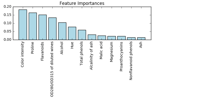
from sklearn.ensemble import RandomForestClassifier
feat_labels = df_wine.columns[1:]   #特征列名
forest = RandomForestClassifier(n_estimators=2000, random_state=0, n_jobs=-1)  #2000棵树,并行工作数是运行服务器决定
forest.fit(X_train, y_train)
importances = forest.feature_importances_   #feature_importances_特征列重要性占比
indices = np.argsort(importances)[::-1]   #对参数从小到大排序的索引序号取逆,即最重要特征索引——>最不重要特征索引
for f in range(X_train.shape[1]):
    print("%2d) %-*s %f" % (f + 1, 30, feat_labels[indices[f]], importances[indices[f]]))   
#-*s表示左对齐字段feat_labels[indices[f]]宽为30
plt.title('Feature Importances')
plt.bar(range(X_train.shape[1]), importances[indices], color='lightblue', align='center')
plt.xticks(range(X_train.shape[1]), feat_labels[indices], rotation=90)
plt.xlim([-1, X_train.shape[1]])
plt.tight_layout()
#plt.savefig('./random_forest.png', dpi=300)
plt.show()
#Output:
# 1) Color intensity                0.183084
# 2) Proline                        0.163305
# 3) Flavanoids                     0.152030
# 4) OD280/OD315 of diluted wines   0.133887
# 5) Alcohol                        0.103847
# 6) Hue                            0.077784
# 7) Total phenols                  0.058778
# 8) Alcalinity of ash              0.031300
# 9) Malic acid                     0.024420
#10) Magnesium                      0.021949
#11) Proanthocyanins                0.021870
#12) Nonflavanoid phenols           0.014450
#13) Ash                            0.013294

if Version(sklearn_version) < '0.18':
    X_selected = forest.transform(X_train, threshold=0.15)
else:
    from sklearn.feature_selection import SelectFromModel
    sfm = SelectFromModel(forest, threshold=0.15, prefit=True)   
    #forest参数是建模完带特征重要性信息的估计器,threshold是特征筛选阈值
    X_selected = sfm.transform(X_train)   #transform对样本X_train进行了选定特征列过滤
X_selected.shape
#Output:
#(124, 3)

for f in range(X_selected.shape[1]):
    print("%2d) %-*s %f" % (f + 1, 30, feat_labels[indices[f]], importances[indices[f]]))
#Output:
# 1) Color intensity                0.183084
# 2) Proline                        0.163305
# 3) Flavanoids                     0.152030