Neural Networks学习笔记

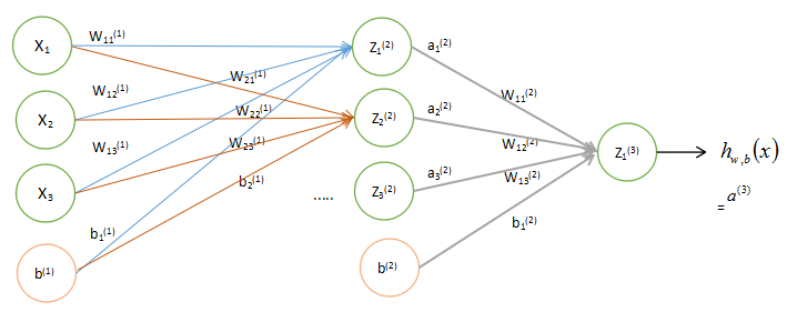
1、神经网络（Neural Networks）

用$n_{l}$表示网络层数，本例中$n_{l}=3$，将第$l$层记为$L_{l}$，于是$L_{1}$是输入层，$L_{n_{l}}$是输出层。本例神经网络有参数 ，其中，，，。
我们用表示第$l$层第$i$单元的激活值（输出值）。当时，也就是第$i$个输入值（输入值的第$i$个特征）。对于给定参数集合$W,b$ ，我们的神经网络就可以按照函数$h_{W,b}(x)$ 来计算输出结果。本例神经网络的计算步骤如下：

我们用$z^{(l)}_i$表示第$l$层第 $i$ 单元输入加权和（包括偏置单元），比如，$z_i^{(2)}$= $\sum_{j=1}^n W^{(1)}_{ij} x_j + b^{(1)}_i$，则 $\textstyle a^{(l)}_i = f(z^{(l)}_i)$。

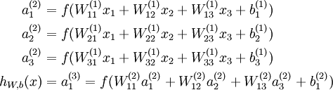
我们将上面的计算步骤叫作前向传播。回想一下，之前我们用 $\textstyle a^{(1)} = x$表示输入层的激活值，那么给定第 $\textstyle l$层的激活值 $\textstyle a^{(l)}$ 后，第 $\textstyle l+1$层的激活值 $\textstyle a^{(l+1)}$ 就可以按照下面步骤计算得到：

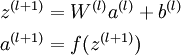
将参数矩阵化，使用矩阵－向量运算方式，我们就可以利用线性代数的优势对神经网络进行快速求解。
其中函数$\textstyle f : \Re \mapsto \Re$ 被称为“激活函数”。通常是sigmoid函数：

它的导数是。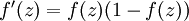
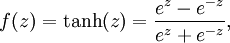
函数是sigmoid函数的一种变体，它的取值范围为 $\textstyle [-1,1]$，而不是sigmoid函数的 $\textstyle [0,1]$。

它的导数是。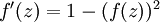

2、反向传导算法（Backpropagation Algorithm）
假设我们有一个固定样本集 $\textstyle \{ (x^{(1)}, y^{(1)})$, $\ldots$, $(x^{(m)}, y^{(m)}) \}$，它包含$\textstyle m$个样例。我们可以用批量梯度下降法来求解神经网络。具体来讲，对于单个样例 $\textstyle (x,y)$，其代价函数为：

$\begin{align} J(W,b; x,y) = \frac{1}{2} \left| h_{W,b}(x) - y \right|^2. \end{align}$
这是一个（二分之一的）方差代价函数。给定一个包含 $\textstyle m$ 个样例的数据集，我们可以定义整体代价函数为：
$\begin{align} J(W,b) &= \left[ \frac{1}{m} \sum_{i=1}^m J(W,b;x^{(i)},y^{(i)}) \right] + \frac{\lambda}{2} \sum_{l=1}^{n_l-1} \; \sum_{i=1}^{s_l} \; \sum_{j=1}^{s_{l+1}} \left( W^{(l)}_{ji} \right)^2 \\ &= \left[ \frac{1}{m} \sum_{i=1}^m \left( \frac{1}{2} \left\| h_{W,b}(x^{(i)}) - y^{(i)} \right\|^2 \right) \right] + \frac{\lambda}{2} \sum_{l=1}^{n_l-1} \; \sum_{i=1}^{s_l} \; \sum_{j=1}^{s_{l+1}} \left( W^{(l)}_{ji} \right)^2 \end{align}$
以上公式中的第一项 $\textstyle J(W,b)$是一个均方差项。第二项是一个规则化项（也叫权重衰减项），其目的是减小权重的幅度，防止过度拟合。
我们的目标是针对参数 $\textstyle W$ 和 $\textstyle b$ 来求其函数 $\textstyle J(W,b)$ 的最小值。为了求解神经网络，我们需要将每一个参数 $\textstyle W^{(l)}_{ij}$和 $\textstyle b^{(l)}_i$初始化为一个很小的、接近零的随机值（比如说，使用正态分布$\textstyle {Normal}(0,\epsilon^2)$生成的随机值，其中 $\textstyle \epsilon$设置为$\textstyle 0.01$），而不是全部置为 $\textstyle$0。如果所有参数都用相同的值作为初始值，那么所有隐藏层单元最终会得到与输入值有关的、相同的函数（也就是说，对于所有 $\textstyle i，\textstyle W^{(1)}_{ij}$都会取相同的值，那么对于任何输入$\textstyle x$都会有：$\textstyle a^{(2)}_1 = a^{(2)}_2 = a^{(2)}_3 = \ldots$）。
梯度下降法中每一次迭代都按照如下公式对参数$\textstyle W$和$\textstyle b$ 进行更新：
$\begin{align} W_{ij}^{(l)} &= W_{ij}^{(l)} - \alpha \frac{\partial}{\partial W_{ij}^{(l)}} J(W,b) \\ b_{i}^{(l)} &= b_{i}^{(l)} - \alpha \frac{\partial}{\partial b_{i}^{(l)}} J(W,b) \end{align}$
其中 $\textstyle \alpha$ 是学习速率。
$\textstyle \frac{\partial}{\partial W_{ij}^{(l)}} J(W,b; x, y)$ 和 $\textstyle \frac{\partial}{\partial b_{i}^{(l)}} J(W,b; x, y)$ 这两项是单个样例 $\textstyle (x,y)$ 的代价函数 $\textstyle J(W,b;x,y)$ 的偏导数。一旦我们求出该偏导数，就可以推导出整体代价函数 $\textstyle J(W,b)$ 的偏导数：
$\begin{align} \frac{\partial}{\partial W_{ij}^{(l)}} J(W,b) &= \left[ \frac{1}{m} \sum_{i=1}^m \frac{\partial}{\partial W_{ij}^{(l)}} J(W,b; x^{(i)}, y^{(i)}) \right] + \lambda W_{ij}^{(l)} \\ \frac{\partial}{\partial b_{i}^{(l)}} J(W,b) &= \frac{1}{m}\sum_{i=1}^m \frac{\partial}{\partial b_{i}^{(l)}} J(W,b; x^{(i)}, y^{(i)}) \end{align}$
反向传播算法的思路如下：给定一个样例$\textstyle (x,y)$，我们首先进行“前向传导”运算，计算出网络中所有的激活值，包括$\textstyle h_{W,b}(x)$ 的输出值。之后，针对第 $\textstyle l$层的每一个节点 $\textstyle i$，我们计算出其“残差” $\textstyle \delta^{(l)}_i$，该残差表明了该节点对最终输出值的残差产生了多少影响。对于最终的输出节点，我们可以直接算出网络产生的激活值与实际值之间的差距，我们将这个差距定义为$\textstyle \delta^{(n_l)}_i$（第 $\textstyle n_l$层表示输出层）。
反向传播算法可表示为以下几个步骤：
1、进行前馈传导计算，利用前向传导公式，得到$\textstyle L_2, L_3, \ldots$直到输出层$\textstyle L_{n_l}$的激活值。
2、对输出层（第 $\textstyle n_l$层），计算：
$\begin{align} \delta^{(n_l)} = - (y - a^{(n_l)}) \bullet f’(z^{(n_l)}) \end{align}（1）$
3、对于$\textstyle l = n_l-1, n_l-2, n_l-3, \ldots, 2$的各层，计算：
$\begin{align} \delta^{(l)} = \left((W^{(l)})^T \delta^{(l+1)}\right) \bullet f’(z^{(l)}) \end{align}（2）$
4、计算最终需要的偏导数值：

$$\begin{align} \nabla_{W^{(l)}} J(W,b;x,y) &= \delta^{(l+1)} (a^{(l)})^T, \\ \nabla_{b^{(l)}} J(W,b;x,y) &= \delta^{(l+1)}.（3） \end{align}$$

假设$\textstyle f(z)$是sigmoid函数，就可以计算得到$\textstyle f'(z^{(l)}_i) = a^{(l)}_i (1- a^{(l)}_i)。$
下面，我们实现批量梯度下降法中的一次迭代：

1、对于所有 $\textstyle l$，令$\textstyle \Delta W^{(l)} := 0$ , $\textstyle \Delta b^{(l)}$ := 0 （设置为全零矩阵或全零向量）
2、对于$\textstyle i = 1$到 $\textstyle m$，
使用反向传播算法计算$\textstyle \nabla_{W^{(l)}} J(W,b;x,y)$ 和 $\textstyle \nabla_{b^{(l)}} J(W,b;x,y)$。
计算$\textstyle \Delta W^{(l)} := \Delta W^{(l)} + \nabla_{W^{(l)}} J(W,b;x,y)$。
计算$\textstyle \Delta b^{(l)} := \Delta b^{(l)} + \nabla_{b^{(l)}} J(W,b;x,y)$。
3、更新权重参数：

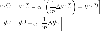
现在，我们可以重复梯度下降法的迭代步骤来减小代价函数$\textstyle J(W,b)$的值，进而求解我们的神经网络。

反向传导算法代码解读
代码来源：Matlab Toolbox for Dimensionality Reduction

function network = backprop(network, X, T, max_iter, noise, lambda)
%BACKPROP Trains a network on a dataset using backpropagation
%
% The function trains the specified network using backpropagation on
% dataset X with targets T for max_iter iterations. The dataset X is an NxD
% matrix, whereas the targets matrix T has size NxM. The function returns 
% the trained network in network.
%targets T作为正确的输出值，用来构建损失函数
%lambda是权重衰减项的系数，一般设置为1e-4
%
    if ~exist('max_iter', 'var') || isempty(max_iter)
        max_iter = 10;
    end
    if ~exist('noise', 'var') || isempty(noise)
        noise = 0;
    end
    if ~exist('lambda', 'var') || isempty(lambda)
        lambda = 0;
    end

    % Initialize some variables
    n = size(X, 1);%X数据集的样本个数
    no_layers = length(network);%网络层数
    batch_size = max(round(n / 100), 100);%选round(n / 100)和100中的大数作为一批样本的容量

    % Perform the backpropagation
    for iter=1:max_iter
        disp([' - iteration ' num2str(iter) ' of ' num2str(max_iter) '...']);

        % Loop over all batches
        index = randperm(n);
        for batch=1:batch_size:n%使用每批样本更新一次W和bias_upW(批量梯度下降法)

            % Select current batch
            tmpX = X(index(batch:min([batch + batch_size - 1 n])),:);%取一批X样本，最后一批不足batch_size的的样本归为一批
            tmpT = T(index(batch:min([batch + batch_size - 1 n])),:);

            % Randomly black out some of the input data
            if noise > 0
                tmpX(rand(size(tmpX)) < noise) = 0;
            end   

            % Convert the weights and store them in the network
            v = [];
            for i=1:length(network)
                v = [v; network{i}.W(:); network{i}.bias_upW(:)];%把所有层的参数W和bias_upW汇总为一个列向量。
            end

            % Conjugate gradient minimization using 3 linesearches
            [v, fX] = minimize(v, 'backprop_gradient', 3, network, tmpX, tmpT, lambda);
            %[C, dC] = backprop_gradient(v, network, X,targets，lambda)
            %使用network和X计算出输出值，与正确输出值targets相减，构建损失函数。lambda是对W进行L2规则化的系数。C是损失函数的值，dC是损失函数的导数值。
            % minimize函数是共轭梯度下降法（3次线性搜索），解决连续可导多变量函数的最优化问题。初始值是参数v（必须是列向量），得到的v使损失函数值最小，即最优值，fX是三次搜索中每次得到的损失函数值（如果搜索不成功，则fX为空）。

            % Deconvert the weights and store them in the network
            ind = 1;%把列向量v拆分成所有层的参数W和bias_upW。
            for i=1:no_layers
                network{i}.W        = reshape(v(ind:ind - 1 + numel(network{i}.W)),        size(network{i}.W));         ind = ind + numel(network{i}.W);
                network{i}.bias_upW = reshape(v(ind:ind - 1 + numel(network{i}.bias_upW)), size(network{i}.bias_upW));  ind = ind + numel(network{i}.bias_upW);
            end

            % Stop upon convergence
            if isempty(fX)
                reconX = run_data_through_autoenc(network, X);
                C = sum((T(:) - reconX(:)) .^ 2) ./ n;
                disp([' - final noisy MSE: ' num2str(C)]);
                return
            end
        end%按批使用样本结束

        % Estimate the current error
        reconX = run_data_through_autoenc(network, X);
        C = sum((T(:) - reconX(:)) .^ 2) ./ n;%估计误差
        disp([' - current noisy MSE: ' num2str(C)]); %每次循环，显示一次误差
    end%达到最大循环次数max_iter

function [X, fX, i] = minimize(X, f, length, P1, P2, P3, P4, P5, P6);

% Minimize a continuous differentialble multivariate function. Starting point
% is given by "X" (D by 1), and the function named in the string "f", must
% return a function value and a vector of partial derivatives. The Polack-
% Ribiere flavour of conjugate gradients is used to compute search directions,
% and a line search using quadratic and cubic polynomial approximations and the
% Wolfe-Powell stopping criteria is used together with the slope ratio method
% for guessing initial step sizes. Additionally a bunch of checks are made to
% make sure that exploration is taking place and that extrapolation will not
% be unboundedly large. The "length" gives the length of the run: if it is
% positive, it gives the maximum number of line searches, if negative its
% absolute gives the maximum allowed number of function evaluations. You can
% (optionally) give "length" a second component, which will indicate the
% reduction in function value to be expected in the first line-search (defaults
% to 1.0). The function returns when either its length is up, or if no further
% progress can be made (ie, we are at a minimum, or so close that due to
% numerical problems, we cannot get any closer). If the function terminates
% within a few iterations, it could be an indication that the function value
% and derivatives are not consistent (ie, there may be a bug in the
% implementation of your "f" function). The function returns the found
% solution "X", a vector of function values "fX" indicating the progress made
% and "i" the number of iterations (line searches or function evaluations,
% depending on the sign of "length") used.
%
% Usage: [X, fX, i] = minimize(X, f, length, P1, P2, P3, P4, P5, P6)
%
% See also: checkgrad 
%
% Copyright (C) 2001 and 2002 by Carl Edward Rasmussen. Date 2002-02-13
%
%

% This file is part of the Matlab Toolbox for Dimensionality Reduction.
% The toolbox can be obtained from http://homepage.tudelft.nl/19j49
% You are free to use, change, or redistribute this code in any way you
% want for non-commercial purposes. However, it is appreciated if you 
% maintain the name of the original author.
%
% (C) Laurens van der Maaten, Delft University of Technology


RHO = 0.01;                            % a bunch of constants for line searches
SIG = 0.5;       % RHO and SIG are the constants in the Wolfe-Powell conditions
INT = 0.1;    % don't reevaluate within 0.1 of the limit of the current bracket
EXT = 3.0;                    % extrapolate maximum 3 times the current bracket
MAX = 20;                         % max 20 function evaluations per line search
RATIO = 100;                                      % maximum allowed slope ratio

argstr = [f, '(X'];                      % compose string used to call function
for i = 1:(nargin - 3)
  argstr = [argstr, ',P', int2str(i)];
end
argstr = [argstr, ')'];                 %构建了语句：backprop_gradient（X,P1，P2，P3，P4）

if max(size(length)) == 2, red=length(2); length=length(1); else red=1; end
if length>0, S=['Linesearch']; else S=['Function evaluation']; end 

i = 0;                                            % zero the run length counter
ls_failed = 0;                             % no previous line search has failed
fX = [];
[f1 df1] = eval(argstr);        %执行之前构建的语句。即，backprop_gradient（X,network, tmpX, tmpT, lambda）
                                                 % get function value and gradient
i = i + (length<0);                                            % count epochs?!
s = -df1;                                        % search direction is steepest
d1 = -s'*s;                                                 % this is the slope
z1 = red/(1-d1);                                  % initial step is red/(|s|+1)

while i < abs(length)                                      % while not finished
  i = i + (length>0);                                      % count iterations?!

  X0 = X; f0 = f1; df0 = df1;                   % make a copy of current values
  X = X + z1*s;                                             % begin line search
  [f2 df2] = eval(argstr);
  i = i + (length<0);                                          % count epochs?!
  d2 = df2'*s;
  f3 = f1; d3 = d1; z3 = -z1;             % initialize point 3 equal to point 1
  if length>0, M = MAX; else M = min(MAX, -length-i); end
  success = 0; limit = -1;                     % initialize quanteties
  while 1
    while ((f2 > f1+z1*RHO*d1) | (d2 > -SIG*d1)) & (M > 0) 
      limit = z1;                                         % tighten the bracket
      if f2 > f1
        z2 = z3 - (0.5*d3*z3*z3)/(d3*z3+f2-f3);                 % quadratic fit
      else
        A = 6*(f2-f3)/z3+3*(d2+d3);                                 % cubic fit
        B = 3*(f3-f2)-z3*(d3+2*d2);
        z2 = (sqrt(B*B-A*d2*z3*z3)-B)/A;       % numerical error possible - ok!
      end
      if isnan(z2) | isinf(z2)
        z2 = z3/2;                  % if we had a numerical problem then bisect
      end
      z2 = max(min(z2, INT*z3),(1-INT)*z3);  % don't accept too close to limits
      z1 = z1 + z2;                                           % update the step
      X = X + z2*s;
      [f2 df2] = eval(argstr);
      M = M - 1; i = i + (length<0);                           % count epochs?!
      d2 = df2'*s;
      z3 = z3-z2;                    % z3 is now relative to the location of z2
    end
    if f2 > f1+z1*RHO*d1 | d2 > -SIG*d1
      break;                                                % this is a failure
    elseif d2 > SIG*d1
      success = 1; break;                                             % success
    elseif M == 0
      break;                                                          % failure
    end
    A = 6*(f2-f3)/z3+3*(d2+d3);                      % make cubic extrapolation
    B = 3*(f3-f2)-z3*(d3+2*d2);
    z2 = -d2*z3*z3/(B+sqrt(B*B-A*d2*z3*z3));        % num. error possible - ok!
    if ~isreal(z2) | isnan(z2) | isinf(z2) | z2 < 0   % num prob or wrong sign?
      if limit < -0.5                               % if we have no upper limit
        z2 = z1 * (EXT-1);                 % the extrapolate the maximum amount
      else
        z2 = (limit-z1)/2;                                   % otherwise bisect
      end
    elseif (limit > -0.5) & (z2+z1 > limit)          % extraplation beyond max?
      z2 = (limit-z1)/2;                                               % bisect
    elseif (limit < -0.5) & (z2+z1 > z1*EXT)       % extrapolation beyond limit
      z2 = z1*(EXT-1.0);                           % set to extrapolation limit
    elseif z2 < -z3*INT
      z2 = -z3*INT;
    elseif (limit > -0.5) & (z2 < (limit-z1)*(1.0-INT))   % too close to limit?
      z2 = (limit-z1)*(1.0-INT);
    end
    f3 = f2; d3 = d2; z3 = -z2;                  % set point 3 equal to point 2
    z1 = z1 + z2; X = X + z2*s;                      % update current estimates
    [f2 df2] = eval(argstr);
    M = M - 1; i = i + (length<0);                             % count epochs?!
    d2 = df2'*s;
  end                                                      % end of line search

  if success                                         % if line search succeeded
    f1 = f2; fX = [fX' f1]';
%     fprintf('%s %6i;  Value %4.6e\r', S, i, f1);
    s = (df2'*df2-df1'*df2)/(df1'*df1)*s - df2;      % Polack-Ribiere direction
    tmp = df1; df1 = df2; df2 = tmp;                         % swap derivatives
    d2 = df1'*s;
    if d2 > 0                                      % new slope must be negative
      s = -df1;                              % otherwise use steepest direction
      d2 = -s'*s;    
    end
    z1 = z1 * min(RATIO, d1/(d2-realmin));          % slope ratio but max RATIO
    d1 = d2;
    ls_failed = 0;                              % this line search did not fail
  else
    X = X0; f1 = f0; df1 = df0;  % restore point from before failed line search
    if ls_failed | i > abs(length)          % line search failed twice in a row
      break;                             % or we ran out of time, so we give up
    end
    tmp = df1; df1 = df2; df2 = tmp;                         % swap derivatives
    s = -df1;                                                    % try steepest
    d1 = -s'*s;
    z1 = 1/(1-d1);                     
    ls_failed = 1;                                    % this line search failed
  end
end

function [C, dC] = backprop_gradient(v, network, X, targets, lambda)
%BACKPROP Compute the cost gradient for CG optimization of a neural network
%为共轭最优化算法构建损失函数和损失函数的梯度
    % Initialize some variables
    n = size(X, 1);
    no_layers = length(network);
    middle_layer = ceil(no_layers / 2);

    % Deconvert the weights and store them in the network
    ind = 1;
    for i=1:no_layers
        network{i}.W        = reshape(v(ind:ind - 1 + numel(network{i}.W)),        size(network{i}.W));         ind = ind + numel(network{i}.W);
        network{i}.bias_upW = reshape(v(ind:ind - 1 + numel(network{i}.bias_upW)), size(network{i}.bias_upW));  ind = ind + numel(network{i}.bias_upW);
    end

    % Run the data through the network
    %前馈传导计算得到网络的各层输出值
    activations = cell(1, no_layers + 1);
    activations{1} = [X ones(n, 1)]; %第一层网络是原始数据X，最后加上一列是bias
    for i=1:no_layers
        if i ~= middle_layer && i ~= no_layers
            activations{i + 1} = [1 ./ (1 + exp(-(activations{i} * [network{i}.W; network{i}.bias_upW]))) ones(n, 1)];%激活函数是sigmiod函数
        else
            activations{i + 1} = [activations{i} * [network{i}.W; network{i}.bias_upW] ones(n, 1)];
        end
    end  

    % Compute value of cost function (= MSE)
    C = (1 / (2 * n)) .* sum(sum((activations{end}(:,1:end - 1) - targets) .^ 2)) + lambda .* sum(v .^ 2);
    %损失函数的第一项是一个均方差项，即网络的输出值activations与正确输出值targets的差。第二项是一个规则化项（也叫权重衰减项），其目的是减小权重v的幅度，防止过度拟合。对应上述文中的J(W,b)
    % Only compute gradient if requested
    if nargout > 1

        % Compute gradients 
        dW = cell(1, no_layers);
        db = cell(1, no_layers);
        Ix = (activations{end}(:,1:end - 1) - targets) ./ n;
        %计算最后一层（输出层）的残差,对应上文中的（1）
        for i=no_layers:-1:1   %从倒数第二层开始，依次计算残差

            % Compute update
            delta = activations{i}' * Ix;%对应上文中的（3），即后一层的残差乘这一层的激活值。（激活值的最后一列为1）
            dW{i} = delta(1:end - 1,:);
            db{i} = delta(end,:);

            % Backpropagate error
            if i > 1
                if i ~= middle_layer + 1
                    Ix = (Ix * [network{i}.W; network{i}.bias_upW]') .* activations{i} .* (1 - activations{i});  %计算各层的残差，对应上文中的（2）
                else
                    Ix = Ix * [network{i}.W; network{i}.bias_upW]';
                end
                Ix = Ix(:,1:end - 1);
            end
        end%所有层的dW，db计算结束

        % Convert gradient information
        %把每层的dW和db汇合成一个列向量dC
        dC = zeros(numel(v), 1);
        ind = 1;
        for i=1:no_layers
            dC(ind:ind - 1 + numel(dW{i})) = dW{i}(:); ind = ind + numel(dW{i});
            dC(ind:ind - 1 + numel(db{i})) = db{i}(:); ind = ind + numel(db{i});
        end
        dC = dC + 2 .* lambda .* v;
    end

参考文献：
UFLDL Tutorial