


相关: KD树+BBF算法解析
SIFT的原理已经有很多大牛的博客上做了解析,本文重点将以Rob Hess等人用C实现的代码做解析,结合代码SIFT原理会更容易理解。一些难理解点的用了☆标注。
欢迎大家批评指正!
转载请注明出处:http://blog.csdn.net/luoshixian099/article/details/47377611
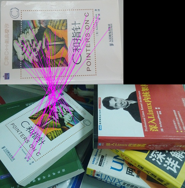
SIFT(Scale-invariant feature transform)即尺度不变特征转换,提取的局部特征点具有尺度不变性,且对于旋转,亮度,噪声等有很高的稳定性。
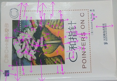
下图中,涉及到图像的旋转,仿射,光照等变化,SIFT算法依然有很好的匹配效果。
SIFT特征点提取
1.图像预处理
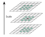
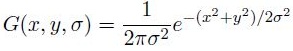
2.构建高斯金字塔(不同尺度下的图像)
3.生成DOG尺度空间
4.关键点搜索与定位
5.计算特征点所在的尺度
6.为特征点分配方向角
7.构建特征描述子
/**
   Finds SIFT features in an image using user-specified parameter values.  All
   detected features are stored in the array pointed to by \a feat.
*/
int _sift_features( IplImage* img, struct feature** feat, int intvls,
		    double sigma, double contr_thr, int curv_thr,
		    int img_dbl, int descr_width, int descr_hist_bins )
{
  IplImage* init_img;
  IplImage*** gauss_pyr, *** dog_pyr;
  CvMemStorage* storage;
  CvSeq* features;
  int octvs, i, n = 0;

  /* check arguments */
  if( ! img )
    fatal_error( "NULL pointer error, %s, line %d",  __FILE__, __LINE__ );
  if( ! feat )
    fatal_error( "NULL pointer error, %s, line %d",  __FILE__, __LINE__ );

  /* build scale space pyramid; smallest dimension of top level is ~4 pixels */
  init_img = create_init_img( img, img_dbl, sigma );                            //对进行图片预处理
  octvs = log( MIN( init_img->width, init_img->height ) ) / log(2) - 2;  //计算高斯金字塔的组数(octave),同时保证顶层至少有4个像素点
  gauss_pyr = build_gauss_pyr( init_img, octvs, intvls, sigma );  //建立高斯金字塔
  dog_pyr = build_dog_pyr( gauss_pyr, octvs, intvls );   //DOG尺度空间

  storage = cvCreateMemStorage( 0 );
  features = scale_space_extrema( dog_pyr, octvs, intvls, contr_thr,   //极值点检测,并去除不稳定特征点
				  curv_thr, storage );
  calc_feature_scales( features, sigma, intvls );                      //计算特征点所在的尺度
  if( img_dbl )
    adjust_for_img_dbl( features );                                       //如果图像初始被扩大了2倍,所有坐标与尺度要除以2
  calc_feature_oris( features, gauss_pyr );                               //计算特征点所在尺度内的方向角
  compute_descriptors( features, gauss_pyr, descr_width, descr_hist_bins );//计算特征描述子 128维向量

  /* sort features by decreasing scale and move from CvSeq to array */
  cvSeqSort( features, (CvCmpFunc)feature_cmp, NULL );   //对特征点按尺度排序
  n = features->total;
  *feat = calloc( n, sizeof(struct feature) );
  *feat = cvCvtSeqToArray( features, *feat, CV_WHOLE_SEQ );
  for( i = 0; i < n; i++ )
    {
      free( (*feat)[i].feature_data );
      (*feat)[i].feature_data = NULL;
    }

  cvReleaseMemStorage( &storage );
  cvReleaseImage( &init_img );
  release_pyr( &gauss_pyr, octvs, intvls + 3 );
  release_pyr( &dog_pyr, octvs, intvls + 2 );
  return n;
}
—————————————————————————————————————————————————————
1.图像预处理
/************************ Functions prototyped here **************************/

/*
  Converts an image to 8-bit grayscale and Gaussian-smooths it.  The image is
  optionally doubled in size prior to smoothing.

  @param img input image
  @param img_dbl if true, image is doubled in size prior to smoothing
  @param sigma total std of Gaussian smoothing
*/
static IplImage* create_init_img( IplImage* img, int img_dbl, double sigma )
{
  IplImage* gray, * dbl;
  double sig_diff;

  gray = convert_to_gray32( img );   //转换为32位灰度图
  if( img_dbl )                                  // 图像被放大二倍
    {
      sig_diff = sqrt( sigma * sigma - SIFT_INIT_SIGMA * SIFT_INIT_SIGMA * 4 );   //  sigma = 1.6 , SIFT_INIT_SIGMA = 0.5  lowe认为图像在尺度0.5下最清晰
      dbl = cvCreateImage( cvSize( img->width*2, img->height*2 ),
			   IPL_DEPTH_32F, 1 );
      cvResize( gray, dbl, CV_INTER_CUBIC );  //双三次插值方法 放大图像
      cvSmooth( dbl, dbl, CV_GAUSSIAN, 0, 0, sig_diff, sig_diff );     //高斯平滑
      cvReleaseImage( &gray );
      return dbl;
    }
  else
    {
      sig_diff = sqrt( sigma * sigma - SIFT_INIT_SIGMA * SIFT_INIT_SIGMA );
      cvSmooth( gray, gray, CV_GAUSSIAN, 0, 0, sig_diff, sig_diff ); // 高斯平滑
      return gray;
    }
}2.构建高斯金字塔
 。
。

 平滑图像,效果是一样的。
/*
Builds Gaussian scale space pyramid from an image
@param base base image of the pyramid
@param octvs number of octaves of scale space
@param intvls number of intervals per octave
@param sigma amount of Gaussian smoothing per octave
@return Returns a Gaussian scale space pyramid as an octvs x (intvls + 3)
array
给定组数(octave)和层数(intvls),以及初始平滑系数sigma,构建高斯金字塔
返回的每组中层数为intvls+3
*/
static IplImage*** build_gauss_pyr( IplImage* base, int octvs,
int intvls, double sigma )
{
IplImage*** gauss_pyr;
const int _intvls = intvls; // lowe 采用了每组层数(intvls)为 3
// double sig_total, sig_prev;
double k;
int i, o;
double *sig = (double *)malloc(sizeof(int)*(_intvls+3)); //存储每组的高斯平滑因子,每组对应的平滑因子都相同
gauss_pyr = calloc( octvs, sizeof( IplImage** ) );
for( i = 0; i < octvs; i++ )
gauss_pyr[i] = calloc( intvls + 3, sizeof( IplImage *) );
/*
precompute Gaussian sigmas using the following formula:
\sigma_{total}^2 = \sigma_{i}^2 + \sigma_{i-1}^2
sig[i] is the incremental sigma value needed to compute
the actual sigma of level i. Keeping track of incremental
sigmas vs. total sigmas keeps the gaussian kernel small.
*/
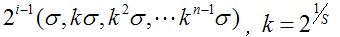
k = pow( 2.0, 1.0 / intvls ); // k = 2^(1/S)
sig[0] = sigma;
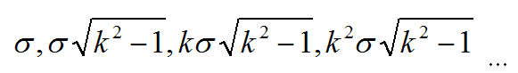
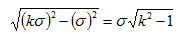
sig[1] = sigma * sqrt( k*k- 1 );
for (i = 2; i < intvls + 3; i++)
sig[i] = sig[i-1] * k; //每组对应的平滑因子为 σ , sqrt(k^2 -1)* σ, sqrt(k^2 -1)* kσ , ...
for( o = 0; o < octvs; o++ )
for( i = 0; i < intvls + 3; i++ )
{
if( o == 0 && i == 0 )
gauss_pyr[o][i] = cvCloneImage(base); //第一组,第一层为原图
/* base of new octvave is halved image from end of previous octave */
else if( i == 0 )
gauss_pyr[o][i] = downsample( gauss_pyr[o-1][intvls] ); //第一层图像由上一层倒数第三张隔点采样得到
/* blur the current octave's last image to create the next one */
else
{
gauss_pyr[o][i] = cvCreateImage( cvGetSize(gauss_pyr[o][i-1]),
IPL_DEPTH_32F, 1 );
cvSmooth( gauss_pyr[o][i-1], gauss_pyr[o][i],
CV_GAUSSIAN, 0, 0, sig[i], sig[i] ); //高斯平滑
}
}
return gauss_pyr;
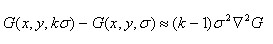
}3.生成DOG尺度空间
 非常近似,且
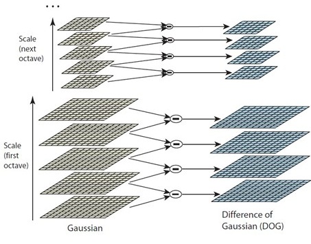
static IplImage*** build_dog_pyr( IplImage*** gauss_pyr, int octvs, int intvls )
{
  IplImage*** dog_pyr;
  int i, o;

  dog_pyr = calloc( octvs, sizeof( IplImage** ) );
  for( i = 0; i < octvs; i++ )
    dog_pyr[i] = calloc( intvls + 2, sizeof(IplImage*) );

  for( o = 0; o < octvs; o++ )
    for( i = 0; i < intvls + 2; i++ )
      {
	dog_pyr[o][i] = cvCreateImage( cvGetSize(gauss_pyr[o][i]),
				       IPL_DEPTH_32F, 1 );
	cvSub( gauss_pyr[o][i+1], gauss_pyr[o][i], dog_pyr[o][i], NULL );   //相邻两层图像相减,结果放在dog_pyr数组内
      }

  return dog_pyr;
}
4.关键点搜索与定位
/*
Detects features at extrema in DoG scale space. Bad features are discarded
based on contrast and ratio of principal curvatures.
@return Returns an array of detected features whose scales, orientations,
and descriptors are yet to be determined.
*/
static CvSeq* scale_space_extrema( IplImage*** dog_pyr, int octvs, int intvls,
double contr_thr, int curv_thr,
CvMemStorage* storage )
{
CvSeq* features;
double prelim_contr_thr = 0.5 * contr_thr / intvls; //极值比较前的阈值处理
struct feature* feat;
struct detection_data* ddata;
int o, i, r, c;
features = cvCreateSeq( 0, sizeof(CvSeq), sizeof(struct feature), storage );
for( o = 0; o < octvs; o++ ) //对DOG尺度空间上,遍历从第二层图像开始到倒数第二层图像上,每个像素点
for( i = 1; i <= intvls; i++ )
for(r = SIFT_IMG_BORDER; r < dog_pyr[o][0]->height-SIFT_IMG_BORDER; r++)
for(c = SIFT_IMG_BORDER; c < dog_pyr[o][0]->width-SIFT_IMG_BORDER; c++)
/* perform preliminary check on contrast */
if( ABS( pixval32f( dog_pyr[o][i], r, c ) ) > prelim_contr_thr ) // 排除像素值小于阈值prelim_contr_thr的点,提高稳定性
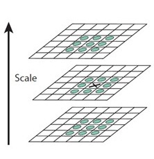
if( is_extremum( dog_pyr, o, i, r, c ) ) //与周围26个像素值比较,是否极大值或者极小值点
{
feat = interp_extremum(dog_pyr, o, i, r, c, intvls, contr_thr); //插值处理,找到准确的特征点坐标
if( feat )
{
ddata = feat_detection_data( feat );
if( ! is_too_edge_like( dog_pyr[ddata->octv][ddata->intvl], //根据Hessian矩阵 判断是否为边缘上的点
ddata->r, ddata->c, curv_thr ) )
{
cvSeqPush( features, feat ); //是特征点进入特征点序列
}
else
free( ddata );
free( feat );
}
}
return features;
}4.1
寻找极值点
/*
  Determines whether a pixel is a scale-space extremum by comparing it to it's
  3x3x3 pixel neighborhood.
*/
static int is_extremum( IplImage*** dog_pyr, int octv, int intvl, int r, int c )
{
  double val = pixval32f( dog_pyr[octv][intvl], r, c );
  int i, j, k;

  /* check for maximum */
  if( val > 0 )
    {
      for( i = -1; i <= 1; i++ )
	for( j = -1; j <= 1; j++ )
	  for( k = -1; k <= 1; k++ )
	    if( val < pixval32f( dog_pyr[octv][intvl+i], r + j, c + k ) )
	      return 0;
    }

  /* check for minimum */
  else
    {
      for( i = -1; i <= 1; i++ )
	for( j = -1; j <= 1; j++ )
	  for( k = -1; k <= 1; k++ )
	    if( val > pixval32f( dog_pyr[octv][intvl+i], r + j, c + k ) )
	      return 0;
    }

  return 1;
}
4.2
准确定位特征点
 ,其中
,其中
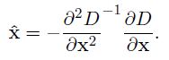
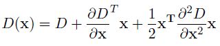
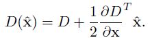 是一个三维矢量,矢量在任何一个方向上的偏移量大于0.5时,意味着已经偏离了原像素点,这样的特征坐标位置需要更新或者继续插值计算。算法实现过程中,为了保证插值能够收敛,设置了最大插值次数(lowe 设置了5次)。同时当
 时(本文阈值采用了0.04/S) ,特征点才被保留,因为响应值过小的点,容易受噪声的干扰而不稳定。
/*
  Performs one step of extremum interpolation.  Based on Eqn. (3) in Lowe's
  paper.

  r,c 为特征点位置,xi,xr,xc,保存三个方向的偏移量
*/

static void interp_step( IplImage*** dog_pyr, int octv, int intvl, int r, int c,
			 double* xi, double* xr, double* xc )
{
  CvMat* dD, * H, * H_inv, X;
  double x[3] = { 0 };

  dD = deriv_3D( dog_pyr, octv, intvl, r, c );      //计算三个方向的梯度
  H = hessian_3D( dog_pyr, octv, intvl, r, c );    // 计算3维空间的hessian矩阵
  H_inv = cvCreateMat( 3, 3, CV_64FC1 );
  cvInvert( H, H_inv, CV_SVD );           //计算逆矩阵
  cvInitMatHeader( &X, 3, 1, CV_64FC1, x, CV_AUTOSTEP );
  cvGEMM( H_inv, dD, -1, NULL, 0, &X, 0 );   //广义乘法

  cvReleaseMat( &dD );
  cvReleaseMat( &H );
  cvReleaseMat( &H_inv );

  *xi = x[2];
  *xr = x[1];
  *xc = x[0];
}
/*
Interpolates a scale-space extremum's location and scale to subpixel
accuracy to form an image feature.
*/
static struct feature* interp_extremum( IplImage*** dog_pyr, int octv, //通过拟合求取准确的特征点位置
int intvl, int r, int c, int intvls,
double contr_thr )
{
struct feature* feat;
struct detection_data* ddata;
double xi, xr, xc, contr;
int i = 0;
while( i < SIFT_MAX_INTERP_STEPS ) //在最大迭代次数范围内进行
{
interp_step( dog_pyr, octv, intvl, r, c, &xi, &xr, &xc ); //插值后得到的三个方向的偏移量(xi,xr,xc)
if( ABS( xi ) < 0.5 && ABS( xr ) < 0.5 && ABS( xc ) < 0.5 )
break;
c += cvRound( xc ); //更新位置
r += cvRound( xr );
intvl += cvRound( xi );
if( intvl < 1 ||
intvl > intvls ||
c < SIFT_IMG_BORDER ||
r < SIFT_IMG_BORDER ||
c >= dog_pyr[octv][0]->width - SIFT_IMG_BORDER ||
r >= dog_pyr[octv][0]->height - SIFT_IMG_BORDER )
{
return NULL;
}
i++;
}
/* ensure convergence of interpolation */
if( i >= SIFT_MAX_INTERP_STEPS )
return NULL;
contr = interp_contr( dog_pyr, octv, intvl, r, c, xi, xr, xc ); //计算插值后对应的函数值
if( ABS( contr ) < contr_thr / intvls ) //小于阈值(0.04/S)的点,则丢弃
return NULL;
feat = new_feature();
ddata = feat_detection_data( feat );
feat->img_pt.x = feat->x = ( c + xc ) * pow( 2.0, octv ); // 计算特征点根据降采样的次数对应于原图中位置
feat->img_pt.y = feat->y = ( r + xr ) * pow( 2.0, octv );
ddata->r = r; // 在本尺度内的坐标位置
ddata->c = c;
ddata->octv = octv; //组信息
ddata->intvl = intvl; // 层信息
ddata->subintvl = xi; // 层方向的偏移量
return feat;
}删除边缘效应
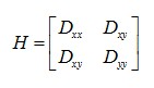
static int is_too_edge_like( IplImage* dog_img, int r, int c, int curv_thr )
{
double d, dxx, dyy, dxy, tr, det;
/* principal curvatures are computed using the trace and det of Hessian */
d = pixval32f(dog_img, r, c); //计算Hessian 矩阵内的4个元素值
dxx = pixval32f( dog_img, r, c+1 ) + pixval32f( dog_img, r, c-1 ) - 2 * d;
dyy = pixval32f( dog_img, r+1, c ) + pixval32f( dog_img, r-1, c ) - 2 * d;
dxy = ( pixval32f(dog_img, r+1, c+1) - pixval32f(dog_img, r+1, c-1) -
pixval32f(dog_img, r-1, c+1) + pixval32f(dog_img, r-1, c-1) ) / 4.0;
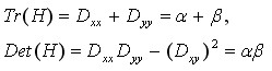
tr = dxx + dyy; //矩阵的迹
det = dxx * dyy - dxy * dxy; //矩阵的值
/* negative determinant -> curvatures have different signs; reject feature */
if( det <= 0 ) // 矩阵值为负值,说明曲率有不同符号,丢弃
return 1;
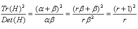
if( tr * tr / det < ( curv_thr + 1.0 )*( curv_thr + 1.0 ) / curv_thr ) //比值小于阈值的特征点被保留 curv_thr = 10
return 0;
return 1;
}5.计算特征点对应的尺度
static void calc_feature_scales( CvSeq* features, double sigma, int intvls )
{
struct feature* feat;
struct detection_data* ddata;
double intvl;
int i, n;
n = features->total;
for( i = 0; i < n; i++ )
{
feat = CV_GET_SEQ_ELEM( struct feature, features, i );
ddata = feat_detection_data( feat );
intvl = ddata->intvl + ddata->subintvl;
feat->scl = sigma * pow( 2.0, ddata->octv + intvl / intvls ); // feat->scl 保存特征点在总体上尺度
ddata->scl_octv = sigma * pow( 2.0, intvl / intvls ); // feat->feature_data->scl__octv 保存特征点在组内的尺度,用来下面计算方向角
}
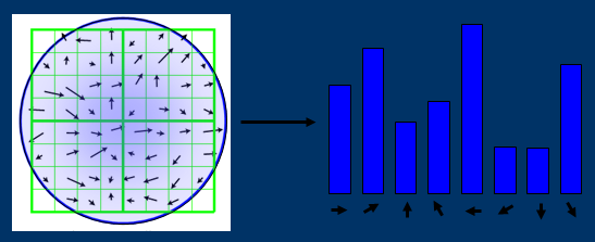
}6.为特征点分配方向角
static void calc_feature_oris( CvSeq* features, IplImage*** gauss_pyr )
{
struct feature* feat;
struct detection_data* ddata;
double* hist;
double omax;
int i, j, n = features->total;
for( i = 0; i < n; i++ )
{
feat = malloc( sizeof( struct feature ) );
cvSeqPopFront( features, feat );
ddata = feat_detection_data( feat );
hist = ori_hist( gauss_pyr[ddata->octv][ddata->intvl], // 计算邻域内的梯度直方图,邻域半径radius = 3*1.5*sigma; 高斯加权系数= 1.5 *sigma
ddata->r, ddata->c, SIFT_ORI_HIST_BINS,
cvRound( SIFT_ORI_RADIUS * ddata->scl_octv ),
SIFT_ORI_SIG_FCTR * ddata->scl_octv );
for( j = 0; j < SIFT_ORI_SMOOTH_PASSES; j++ )
smooth_ori_hist( hist, SIFT_ORI_HIST_BINS ); // 对直方图平滑
omax = dominant_ori( hist, SIFT_ORI_HIST_BINS ); // 返回直方图的主方向
add_good_ori_features( features, hist, SIFT_ORI_HIST_BINS,//大于主方向的80%为辅方向
omax * SIFT_ORI_PEAK_RATIO, feat );
free( ddata );
free( feat );
free( hist );
}
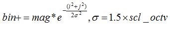
}6.1
建立特征点邻域内的直方图
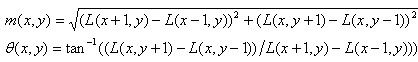
static double* ori_hist( IplImage* img, int r, int c, int n, int rad,
			 double sigma )
{
  double* hist;
  double mag, ori, w, exp_denom, PI2 = CV_PI * 2.0;
  int bin, i, j;

  hist = calloc( n, sizeof( double ) );
  exp_denom = 2.0 * sigma * sigma;
  for( i = -rad; i <= rad; i++ )
    for( j = -rad; j <= rad; j++ )
      if( calc_grad_mag_ori( img, r + i, c + j, &mag, &ori ) )    //计算领域像素点的梯度幅值mag与方向ori
	{
	  w = exp( -( i*i + j*j ) / exp_denom );                    //高斯权重
	  bin = cvRound( n * ( ori + CV_PI ) / PI2 );
	  bin = ( bin < n )? bin : 0;
	  hist[bin] += w * mag;                             //直方图上累加
	}

  return hist;  //返回累加完成的直方图
}平滑直方图
static void smooth_ori_hist( double* hist, int n )
{
  double prev, tmp, h0 = hist[0];
  int i;

  prev = hist[n-1];
  for( i = 0; i < n; i++ )
    {
      tmp = hist[i];
      hist[i] = 0.25 * prev + 0.5 * hist[i] +
	0.25 * ( ( i+1 == n )? h0 : hist[i+1] );
      prev = tmp;
    }
}复制特征点
static void add_good_ori_features( CvSeq* features, double* hist, int n,
				   double mag_thr, struct feature* feat )
{
  struct feature* new_feat;
  double bin, PI2 = CV_PI * 2.0;
  int l, r, i;

  for( i = 0; i < n; i++ )                   //检查所有的方向
    {
      l = ( i == 0 )? n - 1 : i-1;
      r = ( i + 1 ) % n;

      if( hist[i] > hist[l]  &&  hist[i] > hist[r]  &&  hist[i] >= mag_thr ) //判断是不是幅方向
	{
	  bin = i + interp_hist_peak( hist[l], hist[i], hist[r] );     //插值离散处理,取得更精确的方向
	  bin = ( bin < 0 )? n + bin : ( bin >= n )? bin - n : bin;
	  new_feat = clone_feature( feat );       //复制特征点
	  new_feat->ori = ( ( PI2 * bin ) / n ) - CV_PI;//  为特征点方向赋值[-180,180]
	  cvSeqPush( features, new_feat );  //
	  free( new_feat );
	}
    }
}
7.构建特征描述子
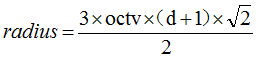
static double*** descr_hist( IplImage* img, int r, int c, double ori,
double scl, int d, int n )
{
double*** hist;
double cos_t, sin_t, hist_width, exp_denom, r_rot, c_rot, grad_mag,
grad_ori, w, rbin, cbin, obin, bins_per_rad, PI2 = 2.0 * CV_PI;
int radius, i, j;
hist = calloc( d, sizeof( double** ) );
for( i = 0; i < d; i++ )
{
hist[i] = calloc( d, sizeof( double* ) );
for( j = 0; j < d; j++ )
hist[i][j] = calloc( n, sizeof( double ) );
}
cos_t = cos( ori );
sin_t = sin( ori );
bins_per_rad = n / PI2;
exp_denom = d * d * 0.5;
hist_width = SIFT_DESCR_SCL_FCTR * scl;
radius = hist_width * sqrt(2) * ( d + 1.0 ) * 0.5 + 0.5; //计算邻域范围半径,+0.5为了取得更多元素
for( i = -radius; i <= radius; i++ )
for( j = -radius; j <= radius; j++ )
{
/*
Calculate sample's histogram array coords rotated relative to ori.
Subtract 0.5 so samples that fall e.g. in the center of row 1 (i.e.
r_rot = 1.5) have full weight placed in row 1 after interpolation.
*/
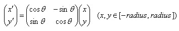
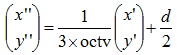
c_rot = ( j * cos_t - i * sin_t ) / hist_width; //
r_rot = ( j * sin_t + i * cos_t ) / hist_width;
rbin = r_rot + d / 2 - 0.5; //旋转后对应的x``及y''
cbin = c_rot + d / 2 - 0.5;
if( rbin > -1.0 && rbin < d && cbin > -1.0 && cbin < d )
if( calc_grad_mag_ori( img, r + i, c + j, &grad_mag, &grad_ori )) //计算每一个像素点的梯度方向、幅值、
{
grad_ori -= ori; //每个像素点相对于特征点的梯度方向
while( grad_ori < 0.0 )
grad_ori += PI2;
while( grad_ori >= PI2 )
grad_ori -= PI2;
obin = grad_ori * bins_per_rad; //像素梯度方向转换成8个方向
w = exp( -(c_rot * c_rot + r_rot * r_rot) / exp_denom ); //每个子区域内像素点,对应的权重
interp_hist_entry( hist, rbin, cbin, obin, grad_mag * w, d, n ); //为了减小突变影响对附近三个bin值三线性插值处理
}
}
return hist;
} ,
这就是128维向量的数据,计算方法
,
这就是128维向量的数据,计算方法
static void interp_hist_entry( double*** hist, double rbin, double cbin,
			       double obin, double mag, int d, int n )
{
  double d_r, d_c, d_o, v_r, v_c, v_o;
  double** row, * h;
  int r0, c0, o0, rb, cb, ob, r, c, o;

  r0 = cvFloor( rbin );
  c0 = cvFloor( cbin );
  o0 = cvFloor( obin );
  d_r = rbin - r0;
  d_c = cbin - c0;
  d_o = obin - o0;

  /*
    The entry is distributed into up to 8 bins.  Each entry into a bin
    is multiplied by a weight of 1 - d for each dimension, where d is the
    distance from the center value of the bin measured in bin units.
  */
  for( r = 0; r <= 1; r++ )
    {
      rb = r0 + r;
      if( rb >= 0  &&  rb < d )
	{
	  v_r = mag * ( ( r == 0 )? 1.0 - d_r : d_r );
	  row = hist[rb];
	  for( c = 0; c <= 1; c++ )
	    {
	      cb = c0 + c;
	      if( cb >= 0  &&  cb < d )
		{
		  v_c = v_r * ( ( c == 0 )? 1.0 - d_c : d_c );
		  h = row[cb];
		  for( o = 0; o <= 1; o++ )
		    {
		      ob = ( o0 + o ) % n;
		      v_o = v_c * ( ( o == 0 )? 1.0 - d_o : d_o );
		      h[ob] += v_o;
		    }
		}
	    }
	}
    }
}static void hist_to_descr( double*** hist, int d, int n, struct feature* feat )
{
int int_val, i, r, c, o, k = 0;
for( r = 0; r < d; r++ )
for( c = 0; c < d; c++ )
for( o = 0; o < n; o++ )
feat->descr[k++] = hist[r][c][o];
feat->d = k;
normalize_descr( feat ); //向量归一化
for( i = 0; i < k; i++ )
if( feat->descr[i] > SIFT_DESCR_MAG_THR ) //设置门限,门限为0.2
feat->descr[i] = SIFT_DESCR_MAG_THR;
normalize_descr( feat ); //向量归一化
/* convert floating-point descriptor to integer valued descriptor */
for( i = 0; i < k; i++ ) //换成整形值
{
int_val = SIFT_INT_DESCR_FCTR * feat->descr[i];
feat->descr[i] = MIN( 255, int_val );
}
}最后对特征点按尺度大小进行排序,强特征点放在前面;
------------------------------------------------------------------------------------
在此非常感谢CSDN上几位图像上的大牛,我也是通过他们的文章去学习研究的,本文也是参考了他们的文章才写成!
推荐看大牛们的文章,原理写的很好!
http://blog.csdn.net/abcjennifer/article/details/7639681
http://blog.csdn.net/zddblog/article/details/7521424
http://blog.csdn.net/chen825919148/article/details/7685952
http://blog.csdn.net/xiaowei_cqu/article/details/8069548


 1245
1245

 被折叠的 条评论
为什么被折叠?
被折叠的 条评论
为什么被折叠?
 到【灌水乐园】发言


