Materials to understand LSTM

本文批评了现有LSTM论文中常见的表述不清及误导性图表,并通过对比不同版本的LSTM架构图,指出了它们的问题所在。作者推荐了一篇优秀的博客文章及其直观的LSTM说明图,同时分享了一个自己绘制的更易于理解的LSTM架构图。

摘要生成于 C知道 ,由 DeepSeek-R1 满血版支持, 前往体验 >

People never judge an academic paper by those user experience standards that they apply to software. If the purpose of a paper were really promoting understanding, then most of them suck. A while ago, I read this article talking about academic pretentiousness and it speaks my heart out. My feeling is, papers are not for better understanding but rather for self-promotion. It’s a way for scholars to declare achievements and make others admire. Therefore the golden standard for an academic paper has always been letting others acknowledge the greatness, but never understand enough to surpass itself.

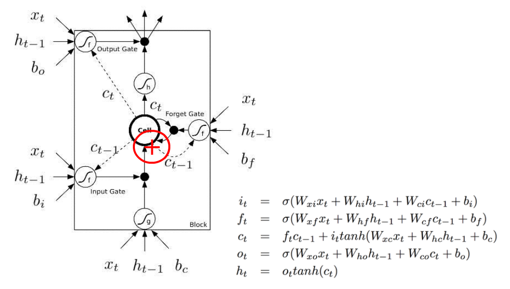
When it comes to LSTM, for example, there aren’t many good materials. Most likely what they would show you is this bullshit image:

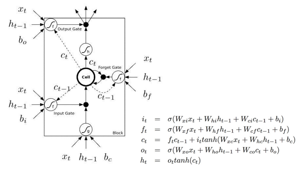
There are many things on this image pisses me off.

First of all, they use these f shapes (with a footnote “f” that looks like a “t”)to denote non-linearity and at the same time, they have f_t in their equations. And they are not the same thing!

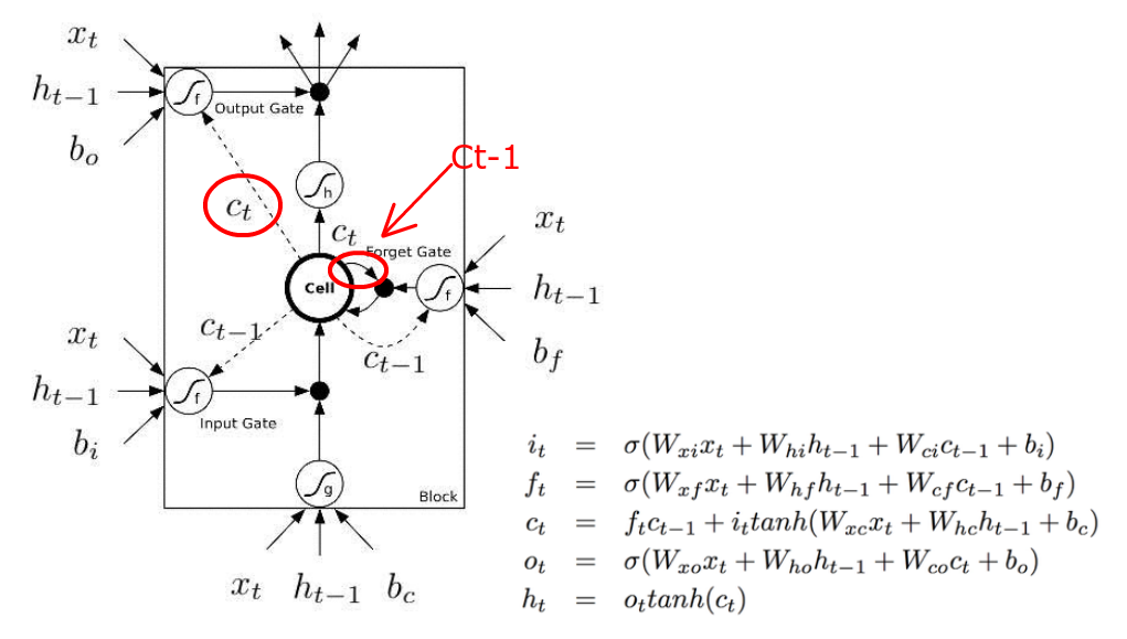
Second, they have these dash lines and solid lines to represent time delay. So solid lines are C_t, and dash lines are C_t-1. There are 5 arrows coming out of the “Cell”, but only 4 are labelled. One C_t is incorrectly labelled with dash line. One solid line is supposed to be a dash line and C_t-1.

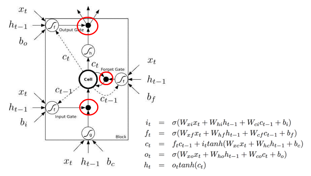
Third, what the hell are black dots? You have to look at the equation to figure out that they are element-wise multiplications of two vectors.

And finally, C_t is supposed to be calculated as a summation of f_t * C_t-1 and i_t * tanh(W_xc * x_t + W_hc*h_t-1 +b_c) (the third equation). But the image completely misses the plus sign.

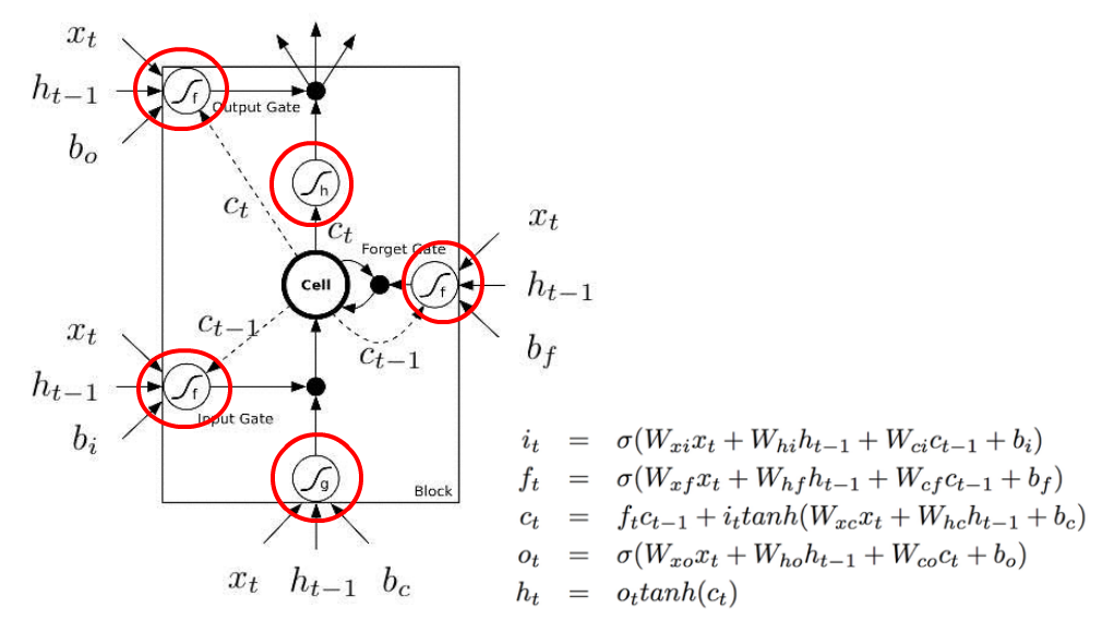
Compared to this shitty image, the following version is slightly better:

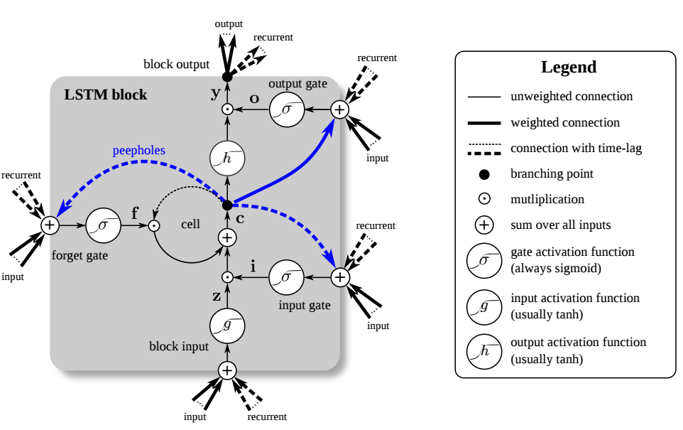
The 3 C_t-1 are correctly represented as dash lines. The plus sign is there too. Sigmoid functions are written with the proper sigma sign, not some freaking f_f.

See, things don’t have to be so difficult. And understanding shouldn’t be a painful experience. But unfortunately, academic writing makes it so almost all the time.

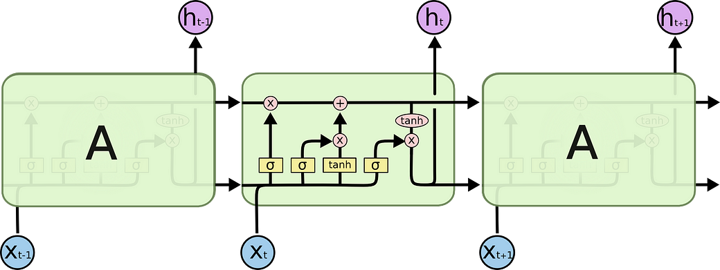
Perhaps the best learning material is really this excellent blog post:

And its diagram is simply beautiful:

I think the most evil thing about the first two versions are that they treat C (the cell, or the memory) not as an input to the LSTM block, but rather a thing that is internal to the block. And they adopt this complex dash line, solid line thing to represent delay. This is really confusing.

But I do noticed one difference between the first two diagrams and the last one. The first two diagrams sum up the inputs with the outputs from the previous layer to calculate the gates (for example, f_t and i_t). But in the third version, the author concatenate them. I don’t know if it is because the third version is a variation or this doesn’t matter in terms of correctness. (But I don’t think it should be concatenation because the vector size h shouldn’t be changed. If it is really concatenation, the vector size of h will change to the size of x+h?)

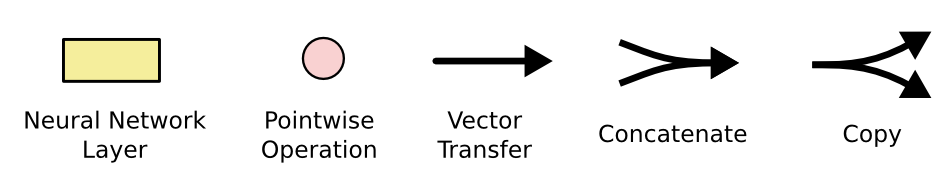
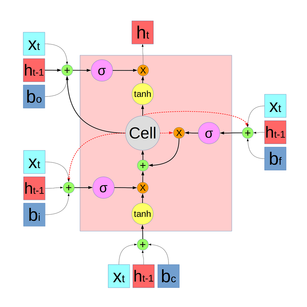
I drew a new diagram, which I think is better:


原文地址: https://medium.com/@shiyan/materials-to-understand-lstm-34387d6454c1

资源下载链接为: https://pan.quark.cn/s/abbae039bf2a 在计算机视觉领域,实时目标跟踪是许多应用的核心任务,例如监控系统、自动驾驶汽车和无人机导航等。本文将重点介绍一种在2017年备受关注的高效目标跟踪算法——BACF(Boosted Adaptive Clustering Filter)。该算法因其卓越的实时性和高精度而脱颖而出,其核心代码是用MATLAB编写的。 BACF算法全称为Boosted Adaptive Clustering Filter,是基于卡尔曼滤波器改进的一种算法。传统卡尔曼滤波在处理复杂背景和目标形变时存在局限性,而BACF通过引入自适应聚类和Boosting策略,显著提升了对目标特征的捕获和跟踪能力。 自适应聚类是BACF算法的关键技术之一。它通过动态更新特征空间中的聚类中心,更准确地捕捉目标的外观变化,从而在光照变化、遮挡和目标形变等复杂情况下保持跟踪的稳定性。此外,BACF还采用了Boosting策略。Boosting是一种集成学习方法,通过组合多个弱分类器形成强分类器。在BACF中,Boosting用于优化目标检测性能,动态调整特征权重,强化对目标识别贡献大的特征,从而提高跟踪精度。BACF算法在设计时充分考虑了计算效率,能够在保持高精度的同时实现快速实时的目标跟踪,这对于需要快速响应的应用场景(如视频监控和自动驾驶)至关重要。 MATLAB作为一种强大的数学计算和数据分析工具,非常适合用于算法的原型开发和测试。BACF算法的MATLAB实现提供了清晰的代码结构,方便研究人员理解其工作原理并进行优化和扩展。通常,BACF的MATLAB源码包含以下部分:主函数(实现整个跟踪算法的核心代码)、特征提取模块(从视频帧中提取目标特征的子程序)、聚类算法(实现自适应聚类过程)、Boosting算法(包含特征权重更新的代
内容概要:本书《Deep Reinforcement Learning with Guaranteed Performance》探讨了基于李雅普诺夫方法的深度强化学习及其在非线性系统最优控制中的应用。书中提出了一种近似最优自适应控制方法,结合泰勒展开、神经网络、估计器设计及滑模控制思想,解决了不同场景下的跟踪控制问题。该方法不仅保证了性能指标的渐近收敛,还确保了跟踪误差的渐近收敛至零。此外,书中还涉及了执行器饱和、冗余解析等问题,并提出了新的冗余解析方法,验证了所提方法的有效性和优越性。 适合人群:研究生及以上学历的研究人员,特别是从事自适应/最优控制、机器人学和动态神经网络领域的学术界和工业界研究人员。 使用场景及目标:①研究非线性系统的最优控制问题,特别是在存在输入约束和系统动力学的情况下;②解决带有参数不确定性的线性和非线性系统的跟踪控制问题;③探索基于李雅普诺夫方法的深度强化学习在非线性系统控制中的应用;④设计和验证针对冗余机械臂的新型冗余解析方法。 其他说明:本书分为七章,每章内容相对独立,便于读者理解。书中不仅提供了理论分析,还通过实际应用(如欠驱动船舶、冗余机械臂)验证了所提方法的有效性。此外,作者鼓励读者通过仿真和实验进一步验证书中提出的理论和技术。
### LSTM细胞状态的可视化 为了更好地理解LSTM的工作机制,尤其是细胞状态的变化过程,可以通过Python中的Matplotlib库和Seaborn库来实现细胞状态的可视化。以下是具体的实现方式: #### 准备工作 首先安装必要的包: ```bash pip install matplotlib seaborn numpy torch ``` 接着导入所需的模块并定义一些辅助函数。 #### 定义LSTM模型结构 基于给定参数构建一个简单的LSTM模型[^3]。 ```python import torch.nn as nn class SimpleLSTM(nn.Module): def __init__(self, input_dim=1, hidden_size_1=128, hidden_size_2=32, stacked_layers=2, dropout_prob=0.5): super(SimpleLSTM, self).__init__() # Encoder part with specified parameters from the reference material. self.encoder_lstm = nn.LSTM(input_dim, hidden_size_1, num_layers=stacked_layers, batch_first=True, dropout=dropout_prob) # Decoder part using different but smaller set of neurons compared to encoder. self.decoder_lstm = nn.LSTM(hidden_size_1, hidden_size_2, num_layers=stacked_layers, batch_first=True, dropout=dropout_prob) def forward(self, x): encoded_output, _ = self.encoder_lstm(x) decoded_output, (hidden_state, _) = self.decoder_lstm(encoded_output) return hidden_state[-1].squeeze() ``` #### 记录细胞状态变化 为了让后续能够绘制出细胞状态随时间演变的情况,在训练过程中保存每次迭代后的细胞状态向量。 #### 数据准备与模拟运行 假设有一个长度为T的时间序列作为输入数据集X,则可以按照如下方式进行处理: ```python import numpy as np import torch def generate_time_series_data(T=100): t = np.linspace(0., 10., T).reshape(-1, 1) X = np.sin(t) * np.exp(-t / 10.) return torch.tensor(X.astype(np.float32)) model = SimpleLSTM() time_steps = [] cell_states = [] with torch.no_grad(): model.eval() data = generate_time_series_data().unsqueeze(dim=-1) outputs, (_, c_t) = model.encoder_lstm(data) for i in range(len(outputs)): time_step = i + 1 cell_state_at_i = c_t[:,i,:].numpy() # Extracting cell states at each step time_steps.append(time_step) cell_states.extend(cell_state_at_i.tolist()) ``` #### 绘制细胞状态图 最后一步就是利用收集到的数据点制作图表展示细胞状态的发展趋势。 ```python import matplotlib.pyplot as plt import seaborn as sns sns.set(style="darkgrid") plt.figure(figsize=(14,7)) ax = sns.lineplot(x=time_steps, y=[item[0] for item in cell_states]) ax.set_title('Visualization of Cell State Evolution Over Time') ax.set_xlabel('Time Step') ax.set_ylabel('Cell State Value') plt.show() ``` 通过上述代码片段,可以看到随着时间推移,细胞状态是如何更新以及其数值范围的大致分布情况。这有助于直观感受LSTM内部运作原理及其记忆特性[^1]。
评论
添加红包

请填写红包祝福语或标题

红包个数最小为10个

红包金额最低5元

当前余额3.43前往充值 >
需支付:10.00
成就一亿技术人!
领取后你会自动成为博主和红包主的粉丝 规则
hope_wisdom
发出的红包
实付
使用余额支付
点击重新获取
扫码支付
钱包余额 0

抵扣说明:

1.余额是钱包充值的虚拟货币,按照1:1的比例进行支付金额的抵扣。
2.余额无法直接购买下载,可以购买VIP、付费专栏及课程。

余额充值