caffe学习笔记10.1--Fine-tuning a Pretrained Network for Style Recognition(new)

在之前的文章里，写过一个关于微调的博客，但是今天上去发现这部分已经更新了http://nbviewer.jupyter.org/github/BVLC/caffe/blob/master/examples/02-fine-tuning.ipynb，因此补一篇最新的，关于微调，前面的文章由讲，参考http://blog.csdn.net/thystar/article/details/50675533

首先，还是需要需要的python导入包：

caffe_root = '../'  # this file should be run from {caffe_root}/examples (otherwise change this line)

import sys
sys.path.insert(0, caffe_root + 'python')
import caffe

caffe.set_device(0)
caffe.set_mode_gpu()

import numpy as np
from pylab import *
%matplotlib inline
import tempfile

下面这个函数用于图像的显示：

def deprocess_net_image(image):
    image = image.copy()              # don't modify destructively
    image = image[::-1]               # BGR -> RGB
    image = image.transpose(1, 2, 0)  # CHW -> HWC
    image += [123, 117, 104]          # (approximately) undo mean subtraction

    # clamp values in [0, 255]
    image[image < 0], image[image > 255] = 0, 255

    # round and cast from float32 to uint8
    image = np.round(image)
    image = np.require(image, dtype=np.uint8)

    return image

1, 设置和数据下载

下载需要的数据：

• get_ilsvrc_aux.sh 下载ImageNet数据集的均值，标签信息
• download_model_binary.py 下载预训练的参数模型
• finetune_flickr_style/assemble_data.py 下载训练和测试数据

与之前一样，我们下载数据中的一个子集，2000张图片，5个类别

# Download just a small subset of the data for this exercise.
# (2000 of 80K images, 5 of 20 labels.)
# To download the entire dataset, set `full_dataset = True`.
full_dataset = False
if full_dataset:
    NUM_STYLE_IMAGES = NUM_STYLE_LABELS = -1
else:
    NUM_STYLE_IMAGES = 2000
    NUM_STYLE_LABELS = 5

# This downloads the ilsvrc auxiliary data (mean file, etc),
# and a subset of 2000 images for the style recognition task.
import os
os.chdir(caffe_root)  # run scripts from caffe root
!data/ilsvrc12/get_ilsvrc_aux.sh
!scripts/download_model_binary.py models/bvlc_reference_caffenet
!python examples/finetune_flickr_style/assemble_data.py \
    --workers=-1  --seed=1701 \
    --images=$NUM_STYLE_IMAGES  --label=$NUM_STYLE_LABELS
# back to examples
os.chdir('examples')

定义权值，引入刚刚下载的权值参数（已训练完成）的路径

import os
weights = caffe_root + 'models/bvlc_reference_caffenet/bvlc_reference_caffenet.caffemodel'
assert os.path.exists(weights)

从 ilsvrc12/synset_words.txt中加载1000个ImageNet数据的标签，从 finetune_flickr_style/style_names.txt里取5个标签

# Load ImageNet labels to imagenet_labels
imagenet_label_file = caffe_root + 'data/ilsvrc12/synset_words.txt'
imagenet_labels = list(np.loadtxt(imagenet_label_file, str, delimiter='\t'))
assert len(imagenet_labels) == 1000
print 'Loaded ImageNet labels:\n', '\n'.join(imagenet_labels[:10] + ['...'])

# Load style labels to style_labels
style_label_file = caffe_root + 'examples/finetune_flickr_style/style_names.txt'
style_labels = list(np.loadtxt(style_label_file, str, delimiter='\n'))
if NUM_STYLE_LABELS > 0:
    style_labels = style_labels[:NUM_STYLE_LABELS]
print '\nLoaded style labels:\n', ', '.join(style_labels)

输出如下：

Loaded ImageNet labels:
n01440764 tench, Tinca tinca
n01443537 goldfish, Carassius auratus
n01484850 great white shark, white shark, man-eater, man-eating shark, Carcharodon carcharias
n01491361 tiger shark, Galeocerdo cuvieri
n01494475 hammerhead, hammerhead shark
n01496331 electric ray, crampfish, numbfish, torpedo
n01498041 stingray
n01514668 cock
n01514859 hen
n01518878 ostrich, Struthio camelus
...

Loaded style labels:
Detailed, Pastel, Melancholy, Noir, HDR

2. 定义和运行网络

这里，用一个函数定义CaffeNet网络结构，指定输入数据和输出类别个数的参数

详细解释下这部分

from caffe import layers as L
from caffe import params as P

定义学习率比率和衰减比率

weight_param = dict(lr_mult=1, decay_mult=1)
bias_param   = dict(lr_mult=2, decay_mult=0)
learned_param = [weight_param, bias_param]

frozen_param = [dict(lr_mult=0)] * 2  #这个变量用于将学习率设置为0，在caffenet中，如果learn_all=False,则使用frozen_param设置网络层的学习率，即学习率为0

定义网络结构

i. 卷积网络与relu激励函数

这里输入参数分别是：

# bottom : 每层的输入

# ks: 卷积核

# nout : 输出神经元个数

# stride: 间隔

# pad : 加边

# group: 组，caffenet卷积部分有分到两个gpu上训练

# param: 学习率参数

# weight_filler: 权值滤波器

# bias_filler: 偏置滤波，一半设为常数

def conv_relu(bottom, ks, nout, stride=1, pad=0, group=1,
              param=learned_param,
              weight_filler=dict(type='gaussian', std=0.01),
              bias_filler=dict(type='constant', value=0.1)):
    conv = L.Convolution(bottom, kernel_size=ks, stride=stride,
                         num_output=nout, pad=pad, group=group,
                         param=param, weight_filler=weight_filler,
                         bias_filler=bias_filler)
    return conv, L.ReLU(conv, in_place=True)

ii. 全连接层

def fc_relu(bottom, nout, param=learned_param,
            weight_filler=dict(type='gaussian', std=0.005),
            bias_filler=dict(type='constant', value=0.1)):
    fc = L.InnerProduct(bottom, num_output=nout, param=param,
                        weight_filler=weight_filler,
                        bias_filler=bias_filler)
    return fc, L.ReLU(fc, in_place=True)

iii. MAX池化层

def max_pool(bottom, ks, stride=1):
    return L.Pooling(bottom, pool=P.Pooling.MAX, kernel_size=ks, stride=stride)

CaffeNet网络结构

def caffenet(data, label=None, train=True, num_classes=1000,
             classifier_name='fc8', learn_all=False):
    """Returns a NetSpec specifying CaffeNet, following the original proto text
       specification (./models/bvlc_reference_caffenet/train_val.prototxt)."""
    n = caffe.NetSpec()
    n.data = data
    param = learned_param if learn_all else frozen_param
    n.conv1, n.relu1 = conv_relu(n.data, 11, 96, stride=4, param=param)
    n.pool1 = max_pool(n.relu1, 3, stride=2)
    n.norm1 = L.LRN(n.pool1, local_size=5, alpha=1e-4, beta=0.75)
    n.conv2, n.relu2 = conv_relu(n.norm1, 5, 256, pad=2, group=2, param=param)
    n.pool2 = max_pool(n.relu2, 3, stride=2)
    n.norm2 = L.LRN(n.pool2, local_size=5, alpha=1e-4, beta=0.75)
    n.conv3, n.relu3 = conv_relu(n.norm2, 3, 384, pad=1, param=param)
    n.conv4, n.relu4 = conv_relu(n.relu3, 3, 384, pad=1, group=2, param=param)
    n.conv5, n.relu5 = conv_relu(n.relu4, 3, 256, pad=1, group=2, param=param)
    n.pool5 = max_pool(n.relu5, 3, stride=2)
    n.fc6, n.relu6 = fc_relu(n.pool5, 4096, param=param)
    if train:
        n.drop6 = fc7input = L.Dropout(n.relu6, in_place=True)
    else:
        fc7input = n.relu6
    n.fc7, n.relu7 = fc_relu(fc7input, 4096, param=param)
    if train:
        n.drop7 = fc8input = L.Dropout(n.relu7, in_place=True)
    else:
        fc8input = n.relu7
    # always learn fc8 (param=learned_param)
    fc8 = L.InnerProduct(fc8input, num_output=num_classes, param=learned_param)
    # give fc8 the name specified by argument `classifier_name`
    n.__setattr__(classifier_name, fc8)
    if not train:
        n.probs = L.Softmax(fc8)
    if label is not None:
        n.label = label
        n.loss = L.SoftmaxWithLoss(fc8, n.label)
        n.acc = L.Accuracy(fc8, n.label)
    # write the net to a temporary file and return its filename
    with tempfile.NamedTemporaryFile(delete=False) as f:
        f.write(str(n.to_proto()))
        return f.name

现在，创建一个“dummy data”(虚拟数据)作为CaffeNet的输入，允许在外部设置输入图像，查看预测类别

dummy_data = L.DummyData(shape=dict(dim=[1, 3, 227, 227]))
imagenet_net_filename = caffenet(data=dummy_data, train=False)
imagenet_net = caffe.Net(imagenet_net_filename, weights, caffe.TEST)

定义一个函数style_net调用caffenet,输入数据参数为Flicker style数据集

• 网络的输入是下载的Flickr style数据集，层类型为ImageData
• 输出是20个类别
• 分类层重命名为fc8_flickr以告诉caffe不要加载原始分类的那一层的权值。

def style_net(train=True, learn_all=False, subset=None):
    if subset is None:
        subset = 'train' if train else 'test'
    source = caffe_root + 'data/flickr_style/%s.txt' % subset
    transform_param = dict(mirror=train, crop_size=227,
        mean_file=caffe_root + 'data/ilsvrc12/imagenet_mean.binaryproto')
    style_data, style_label = L.ImageData(
        transform_param=transform_param, source=source,
        batch_size=50, new_height=256, new_width=256, ntop=2)
    return caffenet(data=style_data, label=style_label, train=train,
                    num_classes=NUM_STYLE_LABELS,
                    classifier_name='fc8_flickr',
                    learn_all=learn_all)

使用style_net初始化未训练的网络， 这个caffeNet的输入图像数据来自于style数据集而其权值来自于之前已经训练好的ImageNet模型

定义untrained_style_net变量调用前向传播函数获取一批训练数据

untrained_style_net = caffe.Net(style_net(train=False, subset='train'),
                                weights, caffe.TEST)
untrained_style_net.forward()
style_data_batch = untrained_style_net.blobs['data'].data.copy()
style_label_batch = np.array(untrained_style_net.blobs['label'].data, dtype=np.int32)

从第一批训练数据的50张图像中选择一张（这里选择第8张）显示该图片，然后在imagenet_net上运行，ImageNet预训练网络给出前5个得分最高的类别

下面我们选择一张网络可以给出合理预测的图片，因为该图像是一张海滩图片，而“沙洲”和“海岸”这两个类别是存在于ImageNet的1000个类别中的，对于其他的图片，预测结果未必好，有些是由于网络识别物体错误，但是跟有可能是由于ImageNet的1000个内别中没有被识别图片的类别。修改batch_index的值将默认的9改为0-49中的任意一个数字，观察其他图像的预测结果。

def disp_preds(net, image, labels, k=5, name='ImageNet'):
    input_blob = net.blobs['data']
    net.blobs['data'].data[0, ...] = image
    probs = net.forward(start='conv1')['probs'][0]
    top_k = (-probs).argsort()[:k]
    print 'top %d predicted %s labels =' % (k, name)
    print '\n'.join('\t(%d) %5.2f%% %s' % (i+1, 100*probs[p], labels[p])
                    for i, p in enumerate(top_k))

def disp_imagenet_preds(net, image):
    disp_preds(net, image, imagenet_labels, name='ImageNet')

def disp_style_preds(net, image):
    disp_preds(net, image, style_labels, name='style')

batch_index = 8
image = style_data_batch[batch_index]
plt.imshow(deprocess_net_image(image))
print 'actual label =', style_labels[style_label_batch[batch_index]]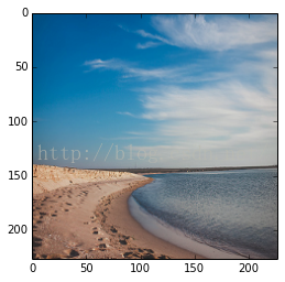

actual label = Melancholy

disp_imagenet_preds(imagenet_net, image)

top 5 predicted ImageNet labels =
        (1) 69.89% n09421951 sandbar, sand bar
        (2) 21.75% n09428293 seashore, coast, seacoast, sea-coast
        (3)  3.22% n02894605 breakwater, groin, groyne, mole, bulwark, seawall, jetty
        (4)  1.89% n04592741 wing
        (5)  1.23% n09332890 lakeside, lakeshore

我们也可以看看 untrained_style_net的预测，但是肯定的不到你感兴趣的结果，因为它还没有开始训练

实际上，因为我们的分类器初始化为0(观察caffenet,没有权值滤波其经过最后的内积层)，softmax的输入应当全部为0，因此，我们看到每个标签的预测结果为1/N,这里n为5，因此所有的预测结果都为20%。

disp_style_preds(untrained_style_net, image)

top 5 predicted style labels =
        (1) 20.00% Detailed
        (2) 20.00% Pastel
        (3) 20.00% Melancholy
        (4) 20.00% Noir
        (5) 20.00% HDR

可以验证在分类层之前的fc7的激励与ImageNet的预训练模型相同（或者十分相似），因为两个模型在conv1到fc7中使用相同的预训练权值

diff = untrained_style_net.blobs['fc7'].data[0] - imagenet_net.blobs['fc7'].data[0]
error = (diff ** 2).sum()
assert error < 1e-8

删除untrained_style_net

del untrained_style_net

3. 训练style分类器

定义solver函数创建caffe的solver文件中的参数，用于训练网络（学习权值），在这个函数中，我们会设置各种参数的值用于学习，显示，和“快照”。这些参数的意思在我之前的博客里都有解释，你可以修改这些值改善预测结果

from caffe.proto import caffe_pb2

def solver(train_net_path, test_net_path=None, base_lr=0.001):
    s = caffe_pb2.SolverParameter()

    # Specify locations of the train and (maybe) test networks.
    s.train_net = train_net_path
    if test_net_path is not None:
        s.test_net.append(test_net_path)
        s.test_interval = 1000  # Test after every 1000 training iterations.
        s.test_iter.append(100) # Test on 100 batches each time we test.

    # The number of iterations over which to average the gradient.
    # Effectively boosts the training batch size by the given factor, without
    # affecting memory utilization.
    s.iter_size = 1
    
    s.max_iter = 100000     # # of times to update the net (training iterations)
    
    # Solve using the stochastic gradient descent (SGD) algorithm.
    # Other choices include 'Adam' and 'RMSProp'.
    s.type = 'SGD'

    # Set the initial learning rate for SGD.
    s.base_lr = base_lr

    # Set `lr_policy` to define how the learning rate changes during training.
    # Here, we 'step' the learning rate by multiplying it by a factor `gamma`
    # every `stepsize` iterations.
    s.lr_policy = 'step'
    s.gamma = 0.1
    s.stepsize = 20000

    # Set other SGD hyperparameters. Setting a non-zero `momentum` takes a
    # weighted average of the current gradient and previous gradients to make
    # learning more stable. L2 weight decay regularizes learning, to help prevent
    # the model from overfitting.
    s.momentum = 0.9
    s.weight_decay = 5e-4

    # Display the current training loss and accuracy every 1000 iterations.
    s.display = 1000

    # Snapshots are files used to store networks we've trained.  Here, we'll
    # snapshot every 10K iterations -- ten times during training.
    s.snapshot = 10000
    s.snapshot_prefix = caffe_root + 'models/finetune_flickr_style/finetune_flickr_style'
    
    # Train on the GPU.  Using the CPU to train large networks is very slow.
    s.solver_mode = caffe_pb2.SolverParameter.GPU
    
    # Write the solver to a temporary file and return its filename.
    with tempfile.NamedTemporaryFile(delete=False) as f:
        f.write(str(s))
        return f.name

现在，我们调用solver函数训练style_net的分类层

这里注意下，如果你想使用命令工具训练网络，命令如下：

build/tools/caffe train \
        -solver models/finetune_flickr_style/solver.prototxt \ 
        -weights models/bvlc_reference_caffenet/bvlc_reference_caffenet.caffemodel \ 
        -gpu 0 

在这里，我们使用python训练这个例子

首先定义run_solvers函数，在这个函数中，给定solvers的列表和步骤的循环。在每一步迭代中记录正确率和损失，最后将学习到的权值保存在一个文件中

def run_solvers(niter, solvers, disp_interval=10):
    """Run solvers for niter iterations,
       returning the loss and accuracy recorded each iteration.
       `solvers` is a list of (name, solver) tuples."""
    blobs = ('loss', 'acc')
    loss, acc = ({name: np.zeros(niter) for name, _ in solvers}
                 for _ in blobs)
    for it in range(niter):
        for name, s in solvers:
            s.step(1)  # run a single SGD step in Caffe
            loss[name][it], acc[name][it] = (s.net.blobs[b].data.copy()
                                             for b in blobs)
        if it % disp_interval == 0 or it + 1 == niter:
            loss_disp = '; '.join('%s: loss=%.3f, acc=%2d%%' %
                                  (n, loss[n][it], np.round(100*acc[n][it]))
                                  for n, _ in solvers)
            print '%3d) %s' % (it, loss_disp)     
    # Save the learned weights from both nets.
    weight_dir = tempfile.mkdtemp()
    weights = {}
    for name, s in solvers:
        filename = 'weights.%s.caffemodel' % name
        weights[name] = os.path.join(weight_dir, filename)
        s.net.save(weights[name])
    return loss, acc, weights

创建和运行solvers训练网络，我们将创建两个方案，一个使用ImageNet的预训练权值初始化（style_solver），另一个使用随机初始化(scratch_style_solver).

在训练过程中，将发现使用预训练的模型更快且有更高的准确率

niter = 200  # number of iterations to train

# Reset style_solver as before.
style_solver_filename = solver(style_net(train=True))
style_solver = caffe.get_solver(style_solver_filename)
style_solver.net.copy_from(weights)

# For reference, we also create a solver that isn't initialized from
# the pretrained ImageNet weights.
scratch_style_solver_filename = solver(style_net(train=True))
scratch_style_solver = caffe.get_solver(scratch_style_solver_filename)

print 'Running solvers for %d iterations...' % niter
solvers = [('pretrained', style_solver),
           ('scratch', scratch_style_solver)]
loss, acc, weights = run_solvers(niter, solvers)
print 'Done.'

train_loss, scratch_train_loss = loss['pretrained'], loss['scratch']
train_acc, scratch_train_acc = acc['pretrained'], acc['scratch']
style_weights, scratch_style_weights = weights['pretrained'], weights['scratch']

# Delete solvers to save memory.
del style_solver, scratch_style_solver, solvers

输出：

Running solvers for 200 iterations...
  0) pretrained: loss=1.609, acc=28%; scratch: loss=1.609, acc=28%
 10) pretrained: loss=1.341, acc=46%; scratch: loss=1.626, acc=14%
 20) pretrained: loss=1.158, acc=58%; scratch: loss=1.641, acc=12%
 30) pretrained: loss=0.869, acc=68%; scratch: loss=1.616, acc=22%
 40) pretrained: loss=0.988, acc=64%; scratch: loss=1.591, acc=24%
 50) pretrained: loss=1.174, acc=62%; scratch: loss=1.610, acc=32%
 60) pretrained: loss=0.871, acc=66%; scratch: loss=1.622, acc=16%
 70) pretrained: loss=1.011, acc=64%; scratch: loss=1.590, acc=30%
 80) pretrained: loss=0.845, acc=66%; scratch: loss=1.593, acc=34%
 90) pretrained: loss=1.090, acc=66%; scratch: loss=1.605, acc=24%
100) pretrained: loss=0.990, acc=64%; scratch: loss=1.589, acc=30%
110) pretrained: loss=1.127, acc=62%; scratch: loss=1.592, acc=30%
120) pretrained: loss=0.886, acc=62%; scratch: loss=1.596, acc=26%
130) pretrained: loss=0.752, acc=70%; scratch: loss=1.586, acc=28%
140) pretrained: loss=0.913, acc=68%; scratch: loss=1.608, acc=18%
150) pretrained: loss=0.493, acc=84%; scratch: loss=1.609, acc=20%
160) pretrained: loss=0.898, acc=70%; scratch: loss=1.597, acc=26%
170) pretrained: loss=1.155, acc=64%; scratch: loss=1.623, acc=20%
180) pretrained: loss=0.904, acc=68%; scratch: loss=1.634, acc=10%
190) pretrained: loss=0.674, acc=74%; scratch: loss=1.610, acc=20%
199) pretrained: loss=0.866, acc=70%; scratch: loss=1.613, acc=14%
Done.

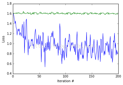
可以看到两种训练过程的正确率和损失。蓝色线条表示使用预训练模型的损失，绿色表示随机初始化的损失。

plot(np.vstack([train_loss, scratch_train_loss]).T)
xlabel('Iteration #')
ylabel('Loss')

输出

<matplotlib.text.Text at 0x7f75d49e1090>

正确率曲线

plot(np.vstack([train_acc, scratch_train_acc]).T)
xlabel('Iteration #')
ylabel('Accuracy')

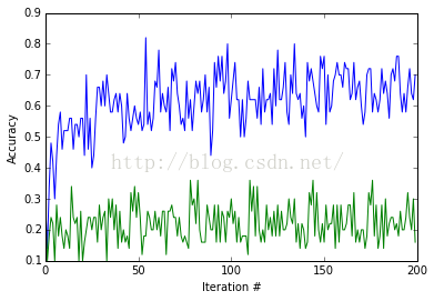
查看这200次迭代的结果，可以看出，预训练的结果要好于随机初始化的结果

def eval_style_net(weights, test_iters=10):
    test_net = caffe.Net(style_net(train=False), weights, caffe.TEST)
    accuracy = 0
    for it in xrange(test_iters):
        accuracy += test_net.forward()['acc']
    accuracy /= test_iters
    return test_net, accuracy

test_net, accuracy = eval_style_net(style_weights)
print 'Accuracy, trained from ImageNet initialization: %3.1f%%' % (100*accuracy, )
scratch_test_net, scratch_accuracy = eval_style_net(scratch_style_weights)
print 'Accuracy, trained from   random initialization: %3.1f%%' % (100*scratch_accuracy, )

Accuracy, trained from ImageNet initialization: 50.0%
Accuracy, trained from   random initialization: 23.6%

4. End-to-End finetuning for style

最后，我们重新训练两个网络，从刚才学习到的权值开始，唯一不同的是，这次权值的学习过程是“end-to-end”的，从RGB conv1滤波器开始，微调网络的所有层。将learn_all参数设为True，这个参数告诉网络将所有层的lr_mult设为一个正数。需要说明的是，可以从前面的代码观察到，tearn_all参数默认值为False,当其为False时，意味着预训练的层（conv1到fc7）的lr_mult=0，我们仅仅学习了最后一层。

注意：两个网络开始的训练进度与之前预训练结束的精度差不多，但是end-to-end的训练由显著的提高

end_to_end_net = style_net(train=True, learn_all=True)

# Set base_lr to 1e-3, the same as last time when learning only the classifier.
# You may want to play around with different values of this or other
# optimization parameters when fine-tuning.  For example, if learning diverges
# (e.g., the loss gets very large or goes to infinity/NaN), you should try
# decreasing base_lr (e.g., to 1e-4, then 1e-5, etc., until you find a value
# for which learning does not diverge).
base_lr = 0.001

style_solver_filename = solver(end_to_end_net, base_lr=base_lr)
style_solver = caffe.get_solver(style_solver_filename)
style_solver.net.copy_from(style_weights)

scratch_style_solver_filename = solver(end_to_end_net, base_lr=base_lr)
scratch_style_solver = caffe.get_solver(scratch_style_solver_filename)
scratch_style_solver.net.copy_from(scratch_style_weights)

print 'Running solvers for %d iterations...' % niter
solvers = [('pretrained, end-to-end', style_solver),
           ('scratch, end-to-end', scratch_style_solver)]
_, _, finetuned_weights = run_solvers(niter, solvers)
print 'Done.'

style_weights_ft = finetuned_weights['pretrained, end-to-end']
scratch_style_weights_ft = finetuned_weights['scratch, end-to-end']

# Delete solvers to save memory.
del style_solver, scratch_style_solver, solvers

输出：
Running solvers for 200 iterations...
  0) pretrained, end-to-end: loss=0.756, acc=76%; scratch, end-to-end: loss=1.585, acc=28%
 10) pretrained, end-to-end: loss=1.286, acc=54%; scratch, end-to-end: loss=1.635, acc=14%
 20) pretrained, end-to-end: loss=1.026, acc=62%; scratch, end-to-end: loss=1.626, acc=12%
 30) pretrained, end-to-end: loss=0.937, acc=68%; scratch, end-to-end: loss=1.597, acc=22%
 40) pretrained, end-to-end: loss=0.745, acc=74%; scratch, end-to-end: loss=1.578, acc=24%
 50) pretrained, end-to-end: loss=0.943, acc=62%; scratch, end-to-end: loss=1.599, acc=34%
 60) pretrained, end-to-end: loss=0.727, acc=74%; scratch, end-to-end: loss=1.555, acc=26%
 70) pretrained, end-to-end: loss=0.625, acc=74%; scratch, end-to-end: loss=1.550, acc=36%
 80) pretrained, end-to-end: loss=0.572, acc=80%; scratch, end-to-end: loss=1.488, acc=48%
 90) pretrained, end-to-end: loss=0.731, acc=68%; scratch, end-to-end: loss=1.497, acc=34%
100) pretrained, end-to-end: loss=0.481, acc=86%; scratch, end-to-end: loss=1.503, acc=32%
110) pretrained, end-to-end: loss=0.512, acc=76%; scratch, end-to-end: loss=1.624, acc=26%
120) pretrained, end-to-end: loss=0.437, acc=82%; scratch, end-to-end: loss=1.534, acc=34%
130) pretrained, end-to-end: loss=0.765, acc=68%; scratch, end-to-end: loss=1.513, acc=30%
140) pretrained, end-to-end: loss=0.439, acc=82%; scratch, end-to-end: loss=1.491, acc=28%
150) pretrained, end-to-end: loss=0.379, acc=84%; scratch, end-to-end: loss=1.489, acc=34%
160) pretrained, end-to-end: loss=0.479, acc=88%; scratch, end-to-end: loss=1.437, acc=30%
170) pretrained, end-to-end: loss=0.467, acc=80%; scratch, end-to-end: loss=1.610, acc=34%
180) pretrained, end-to-end: loss=0.444, acc=82%; scratch, end-to-end: loss=1.471, acc=40%
190) pretrained, end-to-end: loss=0.431, acc=82%; scratch, end-to-end: loss=1.435, acc=42%
199) pretrained, end-to-end: loss=0.483, acc=78%; scratch, end-to-end: loss=1.384, acc=46%
Done.

测试微调后的模型，因为所有的网络参与了识别任务，所以两个网络的结果要好于之前的结果。

test_net, accuracy = eval_style_net(style_weights_ft)
print 'Accuracy, finetuned from ImageNet initialization: %3.1f%%' % (100*accuracy, )
scratch_test_net, scratch_accuracy = eval_style_net(scratch_style_weights_ft)
print 'Accuracy, finetuned from   random initialization: %3.1f%%' % (100*scratch_accuracy, )

Accuracy, finetuned from ImageNet initialization: 53.6%
Accuracy, finetuned from   random initialization: 39.2%

看一下对一开始的那张图像的预测

plt.imshow(deprocess_net_image(image))
disp_style_preds(test_net, image)

top 5 predicted style labels =
	(1) 55.67% Melancholy
	(2) 27.21% HDR
	(3) 16.46% Pastel
	(4)  0.63% Detailed
	(5)  0.03% Noir

看起来要比之前的好，但是，这张图像在测试集中，网络知道这张图片的标签

最后，我们选一张测试集中的图片

batch_index = 1
image = test_net.blobs['data'].data[batch_index]
plt.imshow(deprocess_net_image(image))
print 'actual label =', style_labels[int(test_net.blobs['label'].data[batch_index])]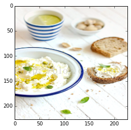

actual label = Pastel

disp_style_preds(test_net, image)

top 5 predicted style labels =
	(1) 99.76% Pastel
	(2)  0.13% HDR
	(3)  0.11% Detailed
	(4)  0.00% Melancholy
	(5)  0.00% Noir

看一下随机初始化的那个网络的结果

disp_style_preds(scratch_test_net, image)

top 5 predicted style labels =
	(1) 49.81% Pastel
	(2) 19.76% Detailed
	(3) 17.06% Melancholy
	(4) 11.66% HDR
	(5)  1.72% Noir

最后，看一下ImageNet的预测结果

disp_imagenet_preds(imagenet_net, image)

top 5 predicted ImageNet labels =
	(1) 34.90% n07579787 plate
	(2) 21.63% n04263257 soup bowl
	(3) 17.75% n07875152 potpie
	(4)  5.72% n07711569 mashed potato
	(5)  5.27% n07584110 consomme

最后，我要说明的是，要注意下第三部分的训练与第四部分的训练的不同，在网络初始化结束后，在系统的tmp目录下面会生成一些临时文件，这些文件包括网络结构和solver文件。在第三次生成的网络结构中，我们可以看到，所有已经预训练的层（conv1-fc7层）lr_mult（学习率的倍数）均为0，而在end-to-end中均是非0正数。

第二个要说明的是，在上一篇关于微调的博客中，使用已经写好的网络结构，新的网络结构与原始的caffenet是有不同的，新的网络中，最后的分类层的学习率的值是原始的caffenet网络的10倍，这个也是网络微调要关注的地方，在我们用已经训练好的模型微调自己的网络结构时，我们只需将变动过的层的学习率调大，关注于训练改动过的那些层。

参考资料：

http://nbviewer.jupyter.org/github/BVLC/caffe/blob/master/examples/02-fine-tuning.ipynb