torch入门笔记13:实现cnn图像分类

这一章主要分享预测的基本操作，并且先将前面分享的内容总结下，完整地实现CNN图像分类的实例

require 'paths'; 
require 'nn'; ---Load TrainSet 
paths.filep("/home/ubuntu64/cifar10torchsmall.zip"); 
trainset = torch.load('cifar10-train.t7'); 
testset = torch.load('cifar10-train.t7'); 
classes = {'airplane', 'automobile', 'bird', 'cat', 'deer', 'dog', 'frog', 'horse', 'ship', 'truck'}; ---Add size() function and Tensor index operator 
setmetatable(trainset, {__index = function(t, i) return {t.data[i], t.label[i]} end} ); trainset.data = trainset.data:double() function 
trainset:size() return self.data:size(1) end 
---Normalize data 
mean = {} 
stdv = {} 
for i=1,3 do
 mean[i] = trainset.data[{ {}, {i}, {}, {} }]:mean()
 print('Channel ' .. i .. ', Mean: ' .. mean[i])
 trainset.data[{ {}, {i}, {}, {} }]:add(-mean[i])
 stdv[i] = trainset.data[{ {}, {i}, {}, {} }]:std()
 print('Channel ' .. i .. ', Standard Deviation:' .. stdv[i])
 trainset.data[{ {}, {i}, {}, {} }]:div(stdv[i])
end

数据的预处理

net = nn.Sequential()

--change 1 channel to 3 channels
--net:add(nn.SpatialConvolution(1, 6, 5, 5))
net:add(nn.SpatialConvolution(3, 6, 5, 5)) 

net:add(nn.ReLU())                       
net:add(nn.SpatialMaxPooling(2,2,2,2))     
net:add(nn.SpatialConvolution(6, 16, 5, 5))
net:add(nn.ReLU())                       
net:add(nn.SpatialMaxPooling(2,2,2,2))
net:add(nn.View(16*5*5))                    
net:add(nn.Linear(16*5*5, 120))         
net:add(nn.ReLU())                       
net:add(nn.Linear(120, 84))
net:add(nn.ReLU())                       
net:add(nn.Linear(84, 10))                  
net:add(nn.LogSoftMax()) 

<span style="font-family: "microsoft yahei"; line-height: 26px; white-space: nowrap; background-color: rgb(255, 255, 255);">与之前建立好的网络有一点不同是将原来的1通道变为3通道，输入的数据集是3通道的彩色图像</span>

criterion = nn.ClassNLLCriterion();

trainer = nn.StochasticGradient(net, criterion)
trainer.learningRate = 0.001
trainer.maxIteration = 5

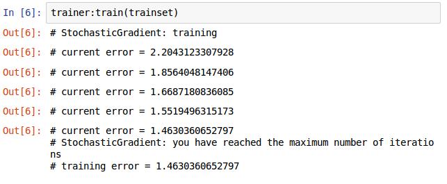
trainer:train(trainset)

<pre name="code" class="html"><span style="font-family: "Source Code Pro", monospace; line-height: 1.45; white-space: nowrap; background-color: rgba(128, 128, 128, 0.0470588);">criterion = nn.ClassNLLCriterion();


trainer = nn.StochasticGradient(net, criterion)
trainer.learningRate = 0.001
trainer.maxIteration = 5


trainer:train(trainset)</span>

训练的过程与前面一样，再重复下，加深印象。 
定义损失函数，选择优化的方法，将网路和损失函数传入，设置学习率和最大迭代次数，开始训练，结果如下图。 
 
现在我们的CNN网络已经训练完了,迭代次数可以多一些，效果不一样，让我测试下看看效果如何。

---

 
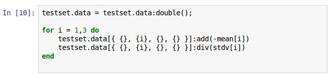
将测试的图像数据用先前的平均值和方差进行同训练集一样的中心化和归一化。 
 
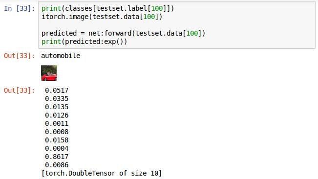
选取第100张图片输入，前两行分别为打印其对应的标签和显示图片，第三行，执行网络的前向传播算法，返回值赋值给predicted。直接打印predicted给出的不是概率而是对数概率。在这十个概率中值最大的为识别的结果，这个是倒数第二个值最大，对应label标签为9，即这张图片被识别成了ship 
 
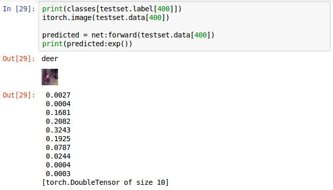
这张最大的是第5个值，即label对应的5，为deer识别正确。 
 
前面的输出的格式还是有些不好，利用torch的sort排序方法将结果排序，返回值中confidences是属于各类的可信度从大到小的排序结果，indices是可信度对应的类的标签，看下打印结果图，一目了然。 
 
 
 
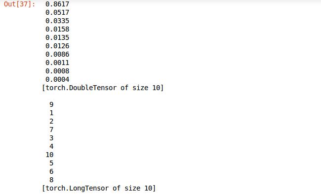
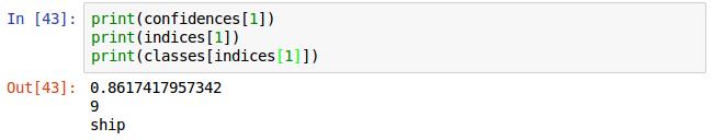
再进一步完善格式，只选取张量的第一个元素打印，并且利用先前定义的classes数组输出名字。 
 
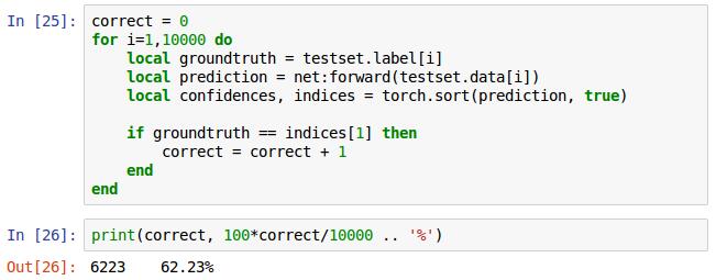
最后是验证总的识别率，for循环，提取测试集中每张照片的标签，每张测试集使用网络net的前向传播forward获得预测结果，将预测结果排序,true表示按递减排序，对比预测结果同真是标签，正确计数器correct加1，将correct除以测试总数10000乘以100得出百分比，这是我迭代10次的正确率为62.23%。 
 
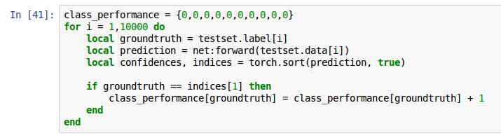
这是统计每类对应的正确率，声明一个数组计数器，用来记录每一类正确识别的个数，改动if语句里面的赋值语句即可完成计数，其他同上。 
 
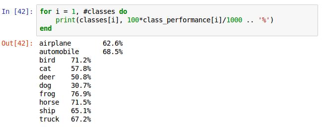
for循环1到classes的数组长度，即10。class_performance[i]里存储的是第i个类的真确识别个数，由于每类有1000张，除以1000，打印结果。

---

预测的源码

--normalize test data
testset.data = testset.data:double();

for i = 1,3 do
    testset.data[{ {}, {i}, {}, {} }]:add(-mean[i])
    testset.data[{ {}, {i}, {}, {} }]:div(stdv[i])
end

--predict test and print confidences
print(classes[testset.label[400]])
itorch.image(testset.data[400])
predicted = net:forward(testset.data[400])
print(predicted:exp())

--sort confidence and print predicted result
confidences, indices = torch.sort(predicted, true)
print(confidences[1])
print(indices[1])
print(classes[indices[1]])

--correct rate in total
correct = 0
for i=1,10000 do
    local groundtruth = testset.label[i]
    local prediction = net:forward(testset.data[i])
    local confidences, indices = torch.sort(prediction, true)

    if groundtruth == indices[1] then
        correct = correct + 1
    end
end

print(correct, 100*correct/10000 .. '%')


--correct rate every class
class_performance = {0,0,0,0,0,0,0,0,0,0}
for i = 1,10000 do
    local groundtruth = testset.label[i]
    local prediction = net:forward(testset.data[i])
    local confidences, indices = torch.sort(prediction, true)

    if groundtruth == indices[1] then
        class_performance[groundtruth] = class_performance[groundtruth] + 1
    end 
end


for i = 1, #classes do 
    print(classes[i], 100*class_performance[i]/1000 .. '%')
end

如果想利用GPU训练该实例用下面的代码替代上文中的训练部分即可

require 'cunn'

net = net:cuda()
criterion = criterion:cuda()
trainset.data = trainset.data:cuda()
trainset.label = trainset.label:cuda()

就可以使用GPU编程。