【python机器学习大作业】基于线性回归的二手房价格预测项目

一、项目介绍

本项目主要对链家二手房房源数据进行分析，通过数据可视化了解广州的二手房源情况，对人们购房做出指导。分析过程主要围绕一下方面展开：项目背景意义、项目结论、项目流程（数据来源、数据可视化与学习、价格估算、线性回归算法）、项目总结。

二、背景意义

2.1 项目背景

在当代中国，随着城市化进程的加速，北、上、广、深等一线城市以其独特的魅力吸引着无数追梦者。广州，作为华南地区的经济中心，不仅经济繁荣，而且文化底蕴深厚，是众多人士梦寐以求的理想居住地。然而，由于一线城市土地资源稀缺，房价高涨，购买一手房对于大多数人来说是一个巨大的挑战。因此，二手房市场成为了众多购房者的首选。

2.2 社会调查反馈

2.2.1 社会情况调查

通过社会调查，我们可以知道一线城市二手房市场回暖，北京深圳二手房成交面积环比增长超过10%，2022年我国6大重点城市二手房成交量第一的是上海市，二手房成交量为15.8万套，其次是成都，二手房成交量为15.13万套，接着是北京市，2022年北京市二手房成交量为14.24万套，然后是广州市，成交量为8.26万套

2.2.2 引用反馈

而我们的二手房价格预测项目能够给用户的带来以下好处：

1. 用户体验
   通过我们的项目，用户们能够快速地了解到心仪房源的价格预测结果，并且这些预测结果与他们实际了解到的市场价格相当接近。同时，系统还提供了丰富的房源信息和筛选功能，使得他们能够更加方便地找到符合自己需求的房源。
2. 决策辅助
   通过我们的系统，用户们能够更加准确地把握市场动态，做出更为合理的购房决策。例如，一些用户原本打算购买新房，但在了解到二手房市场的价格优势和稳定性后，转而选择了二手房。
3. 行业影响
   项目也在一定程度上推动了二手房市场的发展。通过提供更加准确和全面的房源信息，我们帮助购房者更好地了解了市场情况，从而促进了市场的透明度和公平性。同时，我们也为二手房中介提供了更加专业的服务工具，提升了他们的服务质量和竞争力。

2.2.3 该算法软件在该领域的应用情况和需求

随着大数据和人工智能技术的不断发展，算法软件在房地产领域的应用也越来越广泛。在二手房市场中，通过收集和分析大量的房源数据，算法软件能够帮助购房者更加准确地了解市场情况，预测房价走势，并提供个性化的购房建议。因此，对于能够提供准确、全面房源信息的算法软件的需求也在不断增加。

2.3 项目目的

本项目旨在通过对广州链家二手房房源的深入分析，为购房者提供全面、准确的房源信息，帮助他们更好地了解广州二手房市场的整体情况，包括不同行政区、户型、朝向、装修等方面的分布情况，进而辅助购房者做出更为明智的购房决策，并给他们提供理想房屋的大致价格范围。
我们将利用线性回归算法构建一个房价预测模型。该模型将基于历史数据学习房价与各影响因素之间的关系，并据此预测未来房价。用户可以通过输入自己的购房需求（如行政区、地段等级、房屋面积、装修程度等），获得自己心仪房源的价格预测结果，从而更加精准地把握市场动态，做出更为合理的购房决策

三、前期准备

3.1 核心技术

爬虫技术、Numpy、pandas、Matplotlib库的使用，数据清洗，数据可视化，线性回归方程

3.2 数据

3.2.1 数据来源

guangzhou.csv（自己爬虫出来的库）

数据来源于链家网站的数据爬取

广州二手房房源信息：

共计11个行政区，每个行政区900，总计数据量9900条；

3.2.2 数据说明：

1. area：行政区（如：天河区）

2. title：房源信息标题

3. community：小区

4. position：地段位置（如：天河北苑）

5. tax：税率相关（如：房本满五年）

6. total_price：总价，单位：万元

7. unit_price：单价，单位：元/平米

8. hourseType：户型（如：三室一厅）

9. hourseSize：面积，单位：平米

10. direction：房间朝向

11. fitment：装修（如：精装，简装）

3.3第三方库

1. BeautifulSoup:
   作用：用于从HTML和XML文件中提取数据。解析HTML文档，查找、导航、修改和解析树中的标签、属性和文本。
2. pandas:
   作用：数据结构（如DataFrame和Series）的数据分析库。用于数据清洗和分析的功能。
3. tqdm:
   作用：可以在Python长循环中添加一个进度提示信息。
4. math:
   作用：提供了对浮点数学运算的基本函数和常量。
5. requests:
   作用：一个用于发送HTTP请求的库，用于爬虫。
6. re:
   作用：正则表达式库，用于字符串的模式匹配和查找。
7. time:
   作用：提供了各种时间相关的函数。
8. os:
   作用：操作系统交互库，提供了与操作系统交互的许多函数，如文件操作、目录管理等。
9. numpy:
   作用：用于处理大型多维数组和矩阵的库，还提供了大量的数学函数来处理数组。
10. matplotlib.pyplot:
    作用：用于创建静态、动态、交互式的可视化图形。
11. seaborn:
    作用：基于matplotlib的数据可视化库，提供了一个高级接口来绘制有吸引力的统计图形。
12. MyLinearRegression:
    是一个自定义的线性回归模型。。
13. sklearn.model_selection:
    作用：scikit-learn库的一部分，提供了用于模型选择和评估的工具，用于将数据集分割为训练集和测试集。

四、项目结论及效果截图展示

4.1 总体概论

总结：
房价（总价）在（20，250]间的房源数量最多，（250,500]房源数量次之，价格特别高的房很少。可以说房价处于正常范围内。
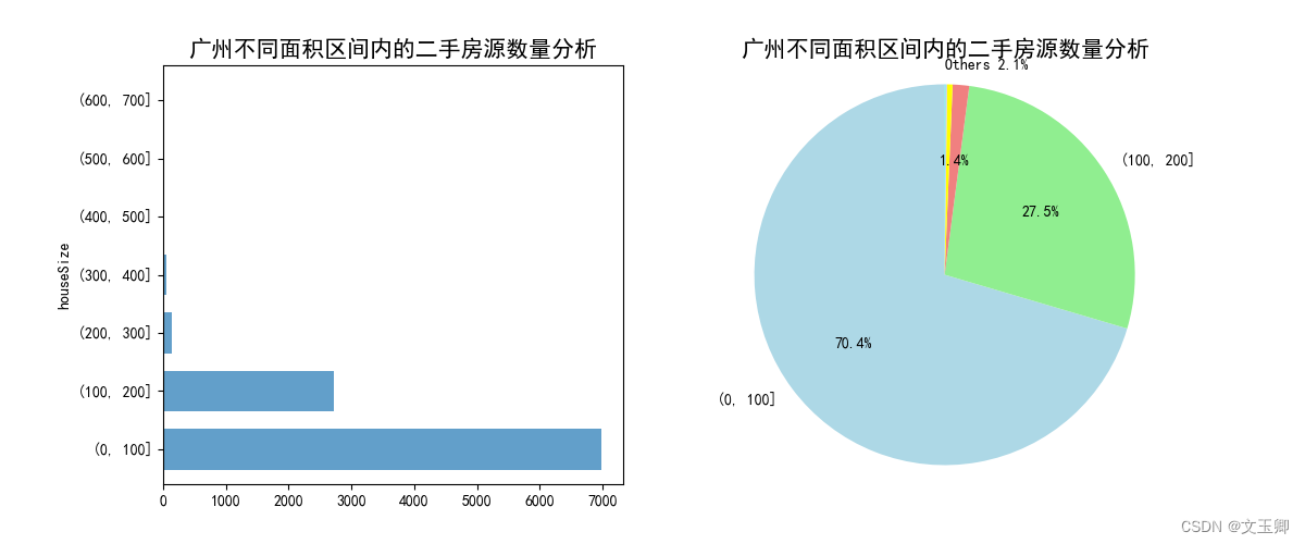
面积（平米）在（0，100]间的房源数量最多，（100,200]房源数量次之，面积特别大的房很少。可以说房屋面积也处于正常范围内。

4.2 影响因素之间的关联

面积houseSize和单位面积房价unit_price的散点图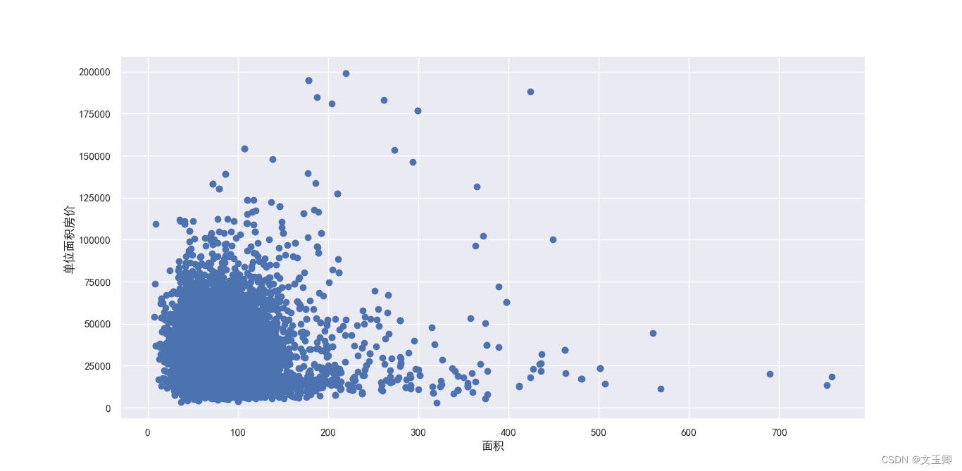
从左到右逐渐稀疏，左密集右稀疏，右偏函数，考虑取对数。
面积houseSize和单位面积房价unit_price（取对数后）的散点图，如下:

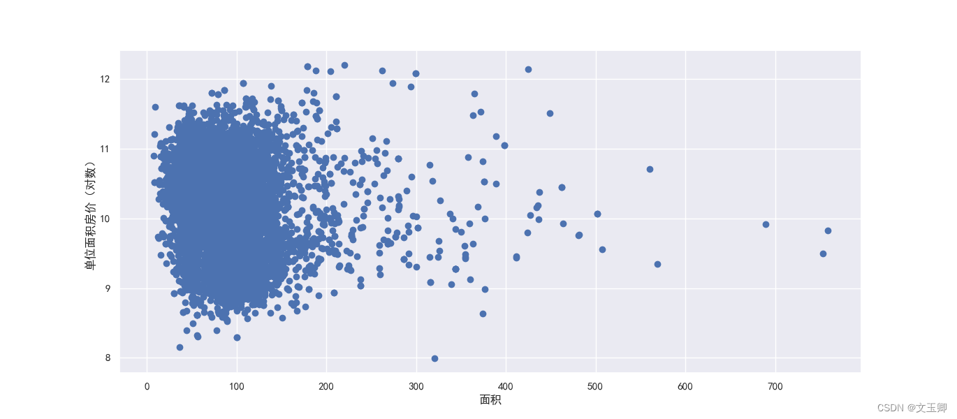
房价取对数后，散点图的结果类似三角关系，散点结果点任比较密
面积houseSize（取对数后）和单位面积房价unit_price（取对数后）的散点图，如下

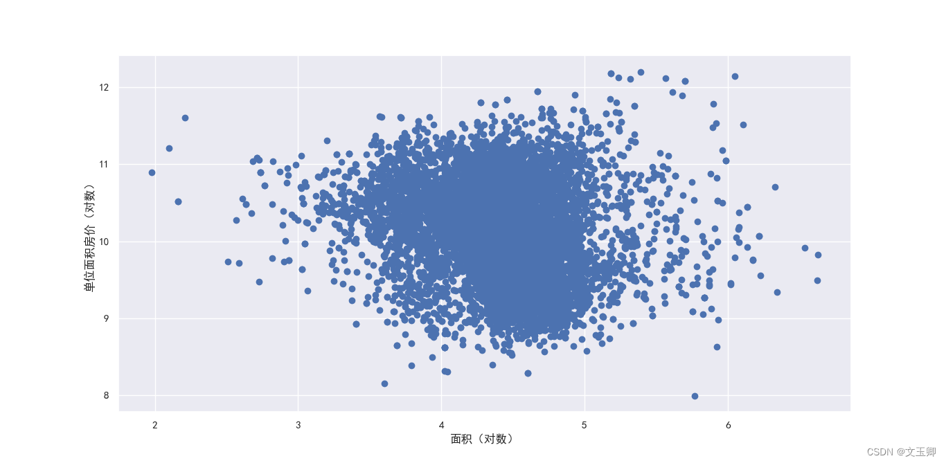
结论：
图形为中间密两边疏的状态，这样的图无论是X分布还是Y分布都是正态分布，同等面积的单位面积房价波动较大。

4.3 影响二手房源价格的因素分析

4.3.1 影响因素：行政区

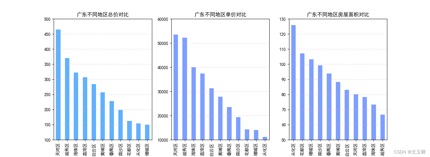
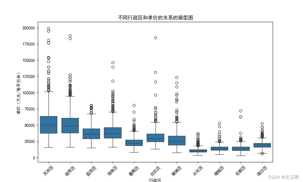
总结：
从以上图形我们可以看出，天河区和越秀区的单价和总价是是11个区中高的，并且其二手房的单价比其他区的都要高1万左右，从化区的单价是最低的。从箱型图可以看出行政区对价格的影响较大。

4.3.2 影响因素：地段

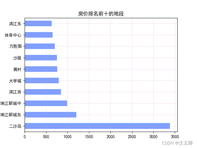
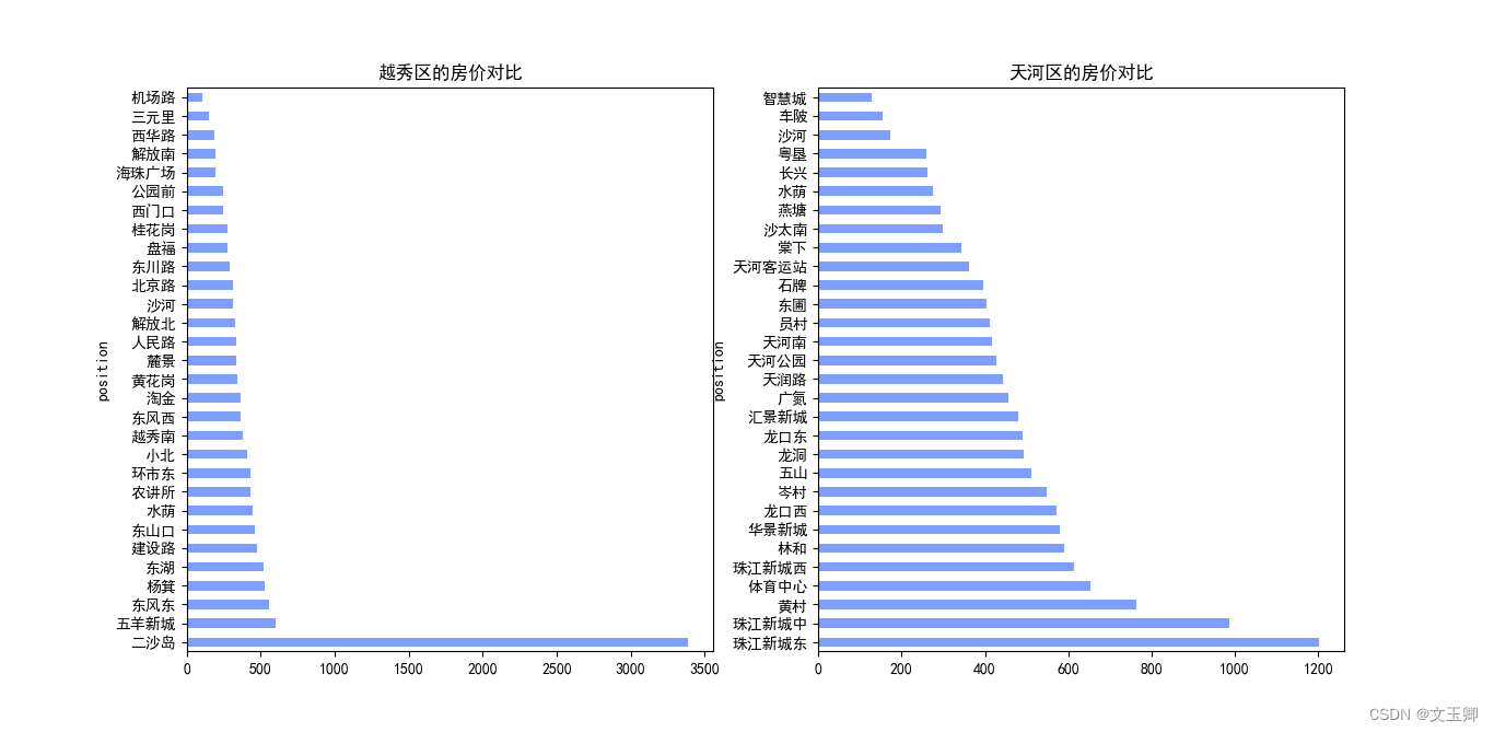
总结：
由以上图形可知，即使在同一个行政区里面，不同地段的价格相差还是挺大的，甚至在越秀区，有着单价近2000的区别，由此可见，地段对单价的影响因素也很大。

4.3.3 影响因素：小区

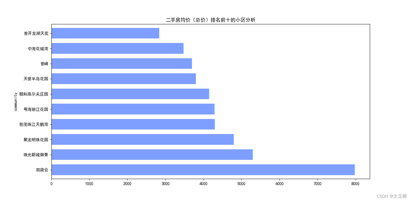
总结：
由以上图形可知，不同小区之间的价格相差还是挺大的，有着单价近3000的区别，但我们并不能排除是因为地段的原因。因此，小区对价格的影响我们暂且定不下论。

4.3.4 影响因素：朝向

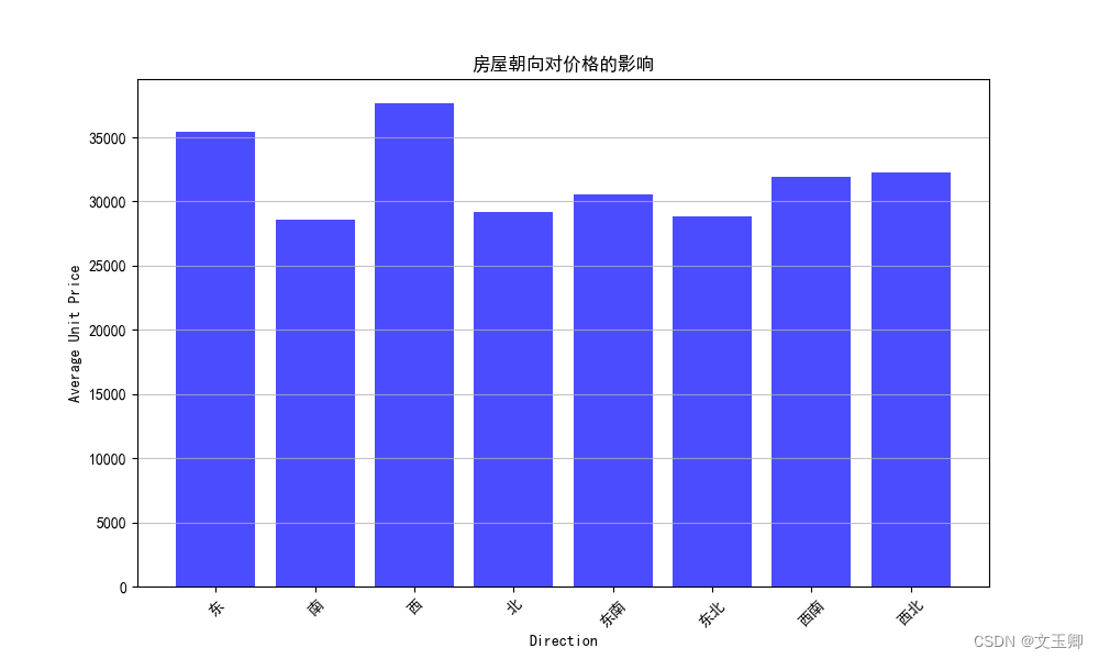
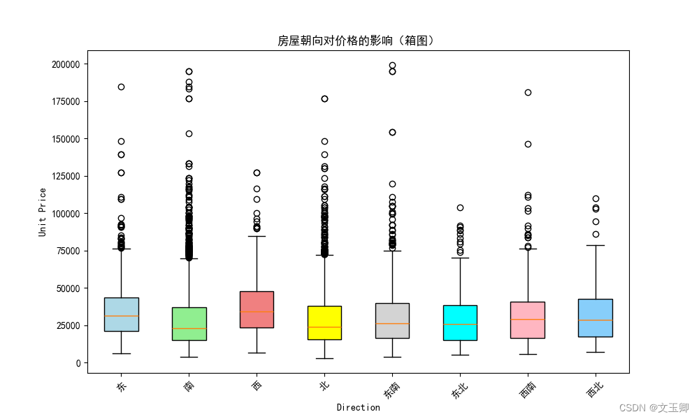
总结：
由以上图形可知，不同朝向之间的价格相差相对较小的，特别是由数据可知一个房屋里面可以不止一个朝向，因此在影响因素中，朝向暂且忽视。

4.3.5 影响因素：装修

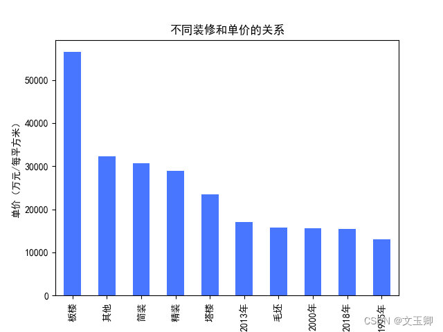
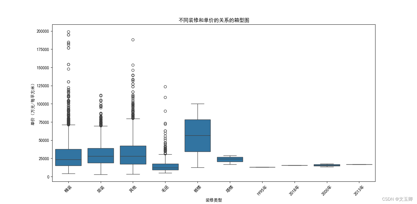
总结：
由以上图形可知，不同装修之间的价格相差还是挺大的，板楼遥遥领先，有着单价近2000的区别。

4.4 价格预测

通过以上结论我们可以知道，影响价格的主要因素为行政区、地段、装修和面积。对此，我通过线性回归算法，做出了一个预测价格的项目。

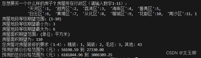
4.4.1 预测项目介绍

该项目要求你输入你想要的行政区、最求地段的等级、房屋面积的需求、以及对装修的需求，来计算你房屋价格单价和总价的范围。

4.4.1 预测精准度

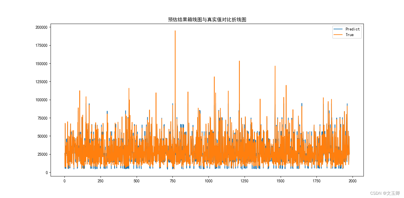
由上图和R方的值，我们可以得知，该算法的预估结果还是相对精确的。

五、全部代码及相关解释

5.1 数据挖掘（data_mining1.py）

这里选择的是链家网站，以广州地区的二手房为例，进行挖掘。

5.1.1 第三方库的引入

from bs4 import BeautifulSoup  
import pandas as pd
from tqdm import tqdm
import math
import requests
import re
import time
import os  

5.1.2 当前文件地址的改变

用于防止后面相对路径保存地址错误

script_dir = os.path.dirname(os.path.abspath(__file__))  
os.chdir(script_dir)  

5.1.3 设置区域变量名

area_dic = {'天河区':'tianhe',
            '越秀区':'yuexiu',
            '荔湾区':'liwan',
            '海珠区':'haizhu',
            '番禺区':'panyu',
            '白云区':'baiyun',
            '黄埔区':'huangpugz',
            '从化区':'conghua',
            '增城区':'zengcheng',
            '花都区':'huadou',
            '南沙区':'nansha'
            }

5.1.4设置header

headers = {'User-Agent': 'Mozilla/5.0 (Windows NT 10.0; Win64; x64) AppleWebKit/537.36 (KHTML, like Gecko) Chrome/65.0.3325.146 Safari/537.36',
           'Referer': 'https://gz.lianjia.com/ershoufang/'}

5.1.4 设置表达式

当表达式匹配失败时，返回默认值（errif）

def re_match(re_pattern, string, errif=None):
    try:
        return re.findall(re_pattern, string)[0].strip()
    except IndexError:
        return errif

5.1.5 数据挖掘

通过requests函数和findall函数将想要的数据爬取出来

#新建一个DataFrame存储信息
data = pd.DataFrame()

for key_, value_ in area_dic.items():
    print('正在搜索{}的二手房信息'.format(key_))
    start_url = 'https://gz.lianjia.com/ershoufang/{}/'.format(value_)
    html = requests.get(start_url,headers=headers).text
    matches = re.findall('共找到<span> (.*?) </span>套.*二手房', html)
    print(matches)
    if matches:  
        house_num = matches[0].strip()  
        print('{}: 二手房源共计「{}」套'.format(key_, house_num))
    else:  
        print("没有找到房源数量信息，有可能跳转到app页面了")
        house_num=1000 
    time.sleep(1)
    # 页面限制 因为广州的行政区太多，如果全都收集的话，爬取时间较久，因此我在这只爬取600条数据。
    minn= min(600,int(house_num))
    total_page = int(math.ceil(minn) / 30.0)
    for i in tqdm(range(total_page), desc=key_):
        #print('开始抓取',url.format(value_, i+1))
        html = requests.get('https://gz.lianjia.com/ershoufang/{}/pg{}/'.format(value_, i+1),headers=headers).text
        soup = BeautifulSoup(html, 'lxml')
        info_collect = soup.find_all(class_="info clear")
        
        for info in info_collect:
            info_dic = {}
            # 行政区
            info_dic['area'] = key_
            # 房源的标题
            info_dic['title'] = re_match('target="_blank">(.*?)</a><!--', str(info))
            # 小区名
            info_dic['community'] = re_match('xiaoqu.*?target="_blank">(.*?)</a>', str(info))
            # 位置
            info_dic['position'] = re_match('<a href.*?target="_blank">(.*?)</a>.*?class="address">', str(info))
            # 税相关，如房本满5年
            info_dic['tax'] = re_match('class="taxfree">(.*?)</span>', str(info))
            try:
                # 总价
                info_dic['total_price'] = float(re_match('<span class="">(.*?)</span><i>万', str(info)))
            except:
                info_dic['total_price'] =None
            # 单价
            try:
                info_dic['unit_price'] = float(re_match('<span>(.*?)元/平</span>', str(info)).replace(',',''))
            except:
                info_dic['unit_price'] =None
            
            # 匹配房源标签信息，通过|切割
            # 包括面积，朝向，装修等信息
            icons = re.findall('class="houseIcon"></span>(.*?)</div>', str(info))[0].strip().split('|')
            info_dic['houseType'] = icons[0].strip()
            info_dic['houseSize'] = float(icons[1].replace('平米', ''))
            info_dic['direction'] = icons[2].strip()
            info_dic['fitment'] = icons[3].strip()
            
            # 存入DataFrame
            if data.empty:
                data = pd.DataFrame(info_dic,index=[0])
            else:
                data1 = pd.DataFrame(info_dic,index=[0])
                data = pd.concat([data,data1],ignore_index=True)

5.1.6 保存数据

将数据保存在和py同个界面下的“guangzhou.csv”文件

try:  
    data.to_csv('./guangzhou.csv') 
    print("数据挖掘成功")  
except Exception as e:  
    print(f"保存失败：{e}")

5.2 数据分析（data_analysis2.py）

5.2.1前提准备

import numpy as np
import pandas as pd 
import matplotlib.pyplot as plt
from pylab import mpl
import os  
import seaborn as sns  

#用于解决中文字体显示问题
plt.rcParams['font.sans-serif'] = ['SimHei']   
plt.rcParams['axes.unicode_minus'] = False  
colors = ['lightblue', 'lightgreen', 'lightcoral', 'yellow', 'lightgray', 'cyan', 'lightpink', 'lightskyblue']    

#将地址改为目前地址，并读取数据
script_dir = os.path.dirname(os.path.abspath(__file__))  
os.chdir(script_dir)  
print(os.getcwd())
df = pd.read_csv('./guangzhou.csv')

因为观察到没有重复数据，所以不用去重

5.2.2了解圳二手房房源的整体情况（总体分析）

（1）平均值观察

#最大值，最小值，平均值等
stats = df.describe() 
print(stats)

（2）数值观察

• 不同户型房源数量占比

# 不同户型房源数量占比
houseType_count = df.groupby('houseType')['houseType'].count()
houseType_count.sort_values(ascending=False,inplace=True)  #按照降序排列
new_houseType_count = houseType_count[houseType_count>10]
new_houseType_count['其它'] = houseType_count[houseType_count<10].sum()
print(new_houseType_count)

• 不同朝向房源数量占比

# 不同朝向房源数量占比
direction_count = df.groupby('direction')['direction'].count()
new_direction_count =direction_count[direction_count>10]
new_direction_count['其它'] = direction_count[direction_count<10].sum()
new_direction_count.sort_values(ascending=False)
print(new_direction_count)

• 不同装修房源数量占比

# 不同装修房源数量占比
fitment_count = df.groupby('fitment')['fitment'].count().sort_values(ascending=False)
fitment_count.sort_values(ascending=False,inplace=True)
print(fitment_count)

（3）绘图观察

• 不同价格区间内的房源数量

# 不同价格区间内的房源数量
fig = plt.figure(figsize=(12,5),dpi=100)
ax1 = fig.add_subplot(1,2,1)
bins_arr = np.arange(0,2500,250)
bins = pd.cut(df['total_price'],bins_arr)
totalprice_counts = df['total_price'].groupby(bins).count()
plt.title("广州不同总价区间内的二手房源数量分析",fontsize=15)
plt.ylabel("二手房数量")
totalprice_counts.plot.barh(alpha=0.7,width=0.7) 

ax2 = fig.add_subplot(1,2,2)
proportions = totalprice_counts / totalprice_counts.sum()  
sorted_indices = proportions.sort_values(ascending=False).index  
top_indices = sorted_indices[:3]  
labels = totalprice_counts.index if len(top_indices) == totalprice_counts.index.size else [''] * len(totalprice_counts.index)  
labels[:len(top_indices)] = totalprice_counts[top_indices].index  
if len(top_indices) < len(sorted_indices):  
    others_proportion = proportions.loc[sorted_indices[len(top_indices):]].sum()  
    labels[-1] = 'Others {:.1%}'.format(others_proportion)  
def my_auopct(pct):
    if (pct<1):  
        return ''  
    else:  
        total = sum(proportions)  
        val = int(round(pct*total/100.0))  
        return '{:1.1f}%'.format(pct) 
ax2.pie(proportions, labels=labels, autopct= my_auopct, colors=colors,  startangle=90)  
ax2.set_title("广州不同总价区间内的二手房源数量分析", fontsize=15)  
plt.show()

• 不同面积区间内的房源数量

# 不同面积区间内的房源数量

fig = plt.figure(figsize=(12,5),dpi=100)
ax1 = fig.add_subplot(1,2,1)
bins_arr = np.arange(0,800,100)
bins = pd.cut(df['houseSize'],bins_arr)
totalprice_counts = df['houseSize'].groupby(bins).count()
plt.title("广州不同面积区间内的二手房源数量分析",fontsize=15)
plt.ylabel("二手房数量")
totalprice_counts.plot.barh(alpha=0.7,width=0.7) 

ax2 = fig.add_subplot(1,2,2)
proportions = totalprice_counts / totalprice_counts.sum()  
sorted_indices = proportions.sort_values(ascending=False).index  
top_indices = sorted_indices[:2]  
labels = totalprice_counts.index if len(top_indices) == totalprice_counts.index.size else [''] * len(totalprice_counts.index)  
labels[:len(top_indices)] = totalprice_counts[top_indices].index  
if len(top_indices) < len(sorted_indices):  
    others_proportion = proportions.loc[sorted_indices[len(top_indices):]].sum()  
    labels[-1] = 'Others {:.1%}'.format(others_proportion)  
def my_auopct(pct):
    if (pct<1): 
        return '' 
    else:  
        total = sum(proportions)  
        val = int(round(pct*total/100.0))  
        return '{:1.1f}%'.format(pct) 
ax2.pie(proportions, labels=labels, autopct= my_auopct, colors=colors,  startangle=90)  
ax2.axis('equal')  
ax2.set_title("广州不同面积区间内的二手房源数量分析", fontsize=15)  
plt.show()

（4）面积与单位价格的关系

# 面积和单面积房价之间的关联
#面积houseSize和单位面积房价unit_price的散点图
plt.figure(figsize=(20,6))
sns.set(font='SimHei')
plt.scatter(x=df.houseSize,y=df.unit_price,marker='o')
plt.xlabel("面积")
plt.ylabel("单位面积房价")
plt.show()
# 从左到右逐渐稀疏，左密集右稀疏，右偏函数，考虑取对数。
#面积houseSize和单位面积房价unit_price（取对数后）的散点图
per=np.log(df['unit_price'])
plt.figure(figsize=(20,6))
sns.set(font='SimHei')
plt.scatter(x=df.houseSize,y=per,marker='o')
plt.xlabel("面积")
plt.ylabel("单位面积房价（对数）")
plt.show()
#房价取对数后，散点图的结果类似三角关系，散点结果点任比较密
#面积houseSize（取对数后）和单位面积房价unit_price（取对数后）的散点图
per=np.log(df['unit_price'])
houseSize=np.log(df['houseSize'])
plt.figure(figsize=(20,8))
sns.set(font='SimHei')
plt.scatter(x=houseSize,y=per,marker='o')
plt.xlabel("面积（对数）")
plt.ylabel("单位面积房价（对数）")
plt.show()
#图形为中间密两边疏的状态，这样的图无论是X分布还是Y分布都是正态分布，同等面积的单位面积房价波动较大。

5.2.3 影响二手房源价格的因素分析

（1）影响因素：行政区

• 数值

#行政区
# 不同区的总价平均值对比
area_house_mean_totalprice = df.groupby('area')['total_price'].mean()
area_house_mean_totalprice.sort_values(ascending=False,inplace=True)
print(area_house_mean_totalprice)

# 不同区的单价平均值对比
area_house_mean_unitprice = df.groupby('area')['unit_price'].mean()
area_house_mean_unitprice.sort_values(ascending=False,inplace=True)
print(area_house_mean_unitprice)

# 不同区的面积平均值对比
area_house_mean_houseSize = df.groupby('area')['houseSize'].mean()
area_house_mean_houseSize.sort_values(ascending=False,inplace=True)
print(area_house_mean_houseSize)

• 直方图

fig = plt.figure(figsize=(15,5),dpi=100)
ax1 = fig.add_subplot(1,3,1)
plt.title("广东不同地区总价对比")
plt.ylim([100,500])  
rects = area_house_mean_totalprice.plot.bar(alpha=0.7,color='#1E90FF')
plt.grid(alpha=0.5,color='#DDA0DD',linestyle='--',axis='y')

ax2 = fig.add_subplot(1,3,2)
plt.title("广东不同地区单价对比")
plt.ylim([10000,60000])
area_house_mean_unitprice.plot.bar(alpha=0.7,color='#4876FF')
plt.grid(alpha=0.5,color='#DDA0DD',linestyle='--',axis='y')

ax2 = fig.add_subplot(1,3,3)
plt.title("广东不同地区房屋面积对比")
plt.ylim([50,130])
area_house_mean_houseSize.plot.bar(alpha=0.7,color='#4876FF')
plt.grid(alpha=0.5,color='#DDA0DD',linestyle='--',axis='y')

• 箱型图

plt.figure(figsize=(10, 6)) 
sns.boxplot(x='area', y='unit_price', data=df)  
plt.title("不同行政区和单价的关系的箱型图")   
plt.xlabel("行政区")  
plt.ylabel("单价（万元/每平方米）")  
plt.xticks(rotation=45)   
plt.show()

（2）影响因素：地段

#不同地段对价格的影响
position_house_mean_price = df.groupby('position')['total_price'].mean()
position_house_mean_price.sort_values(ascending=False,inplace=True)
ax = plt.subplot(111)
plt.title("房价排名前十的地段") 
position_house_mean_price.head(10).plot.barh(alpha=0.7,color='#4876FF')
plt.grid(color='#DDA0DD',linestyle='--',alpha=0.5)
plt.show()

因为前十的地段可能无法体现出地段的影响，所以下面用了同一行政区的不同地段来观察

# 越秀区的不同地段的均价对比
area_nanshan_price = df[df['area']=='越秀区'].groupby('position')['total_price'].mean()
area_nanshan_price.sort_values(ascending=False,inplace=True)
# 天河区的不同地段的均价对比
area_baoan_price = df[df['area']=='天河区'].groupby('position')['total_price'].mean()
area_baoan_price.sort_values(ascending=False,inplace=True)
fig = plt.figure(figsize=(15,8),dpi=100)
ax1 = fig.add_subplot(1,2,1)
plt.title("越秀区的房价对比")
area_nanshan_price.plot.barh(alpha=0.7,color=colors) 
ax2 = fig.add_subplot(1,2,2)
plt.title("天河区的房价对比")
area_baoan_price.plot.barh(alpha=0.7,color=colors) 
plt.show() 

（3）影响因素：小区

#小区对价格的影响
community_top10 = df.groupby('community')['total_price'].mean().sort_values(ascending=False).head(10)
ax = plt.subplot(111)
plt.title("二手房均价（总价）排名前十的小区分析")
community_top10.plot.barh(alpha=0.7,width=0.7,color='#4876FF')
plt.show()

（4）影响因素：朝向

• 直方图

# 定义方向列表  
directions = ['东', '南', '西', '北', '东南', '东北', '西南', '西北']  
direction_prices = {direction: [] for direction in directions}  
for index, row in df.iterrows():  
    directions_in_house = row['direction'].split()  
    for direction in directions_in_house:  
        if direction in directions:  
            direction_prices[direction].append(row['unit_price'])  
  
# 计算每个方向的平均价格  
direction_avg_prices = {direction: sum(prices) / len(prices) if prices else 0 for direction, prices in direction_prices.items()}   
result_df = pd.DataFrame(list(direction_avg_prices.items()), columns=['Direction', 'Average Price'])  
  
# 绘制直方图  
plt.figure(figsize=(10, 6))  
plt.bar(result_df['Direction'], result_df['Average Price'], color='blue', alpha=0.7)  
plt.title("房屋朝向对价格的影响")  
plt.xlabel("Direction")  
plt.ylabel("Average Unit Price")  
plt.xticks(rotation=45)  
plt.grid(axis='y', alpha=0.75)  
plt.show()

• 箱型图

#绘制箱型图
fig, ax = plt.subplots(figsize=(10, 6))    
bp = ax.boxplot(list(direction_prices.values()), patch_artist=True)  
ax.set_xticklabels(directions, rotation=45)  
ax.set_title("房屋朝向对价格的影响（箱图）")  
ax.set_xlabel("Direction")  
ax.set_ylabel("Unit Price")  
for patch, color in zip(bp['boxes'], colors):  
    patch.set_facecolor(color)    
plt.show()

（5）影响因素：房屋装修

• 直方图

#装修对价格的影响
df_filtered = df[df['fitment'] != '暂无数据']  
fit_price = df_filtered.groupby('fitment')['unit_price'].mean().sort_values(ascending=False)
ax = plt.subplot(111)
plt.title("不同装修和单价的关系")
plt.ylabel("单价（万元/每平方米）")
fit_price.plot.bar(color='#4876FF')
plt.show()

• 箱型图

# 使用Seaborn库来绘制箱型图  
plt.figure(figsize=(10, 6)) 
sns.boxplot(x='fitment', y='unit_price', data=df_filtered)  
plt.title("不同装修和单价的关系的箱型图")   
plt.xlabel("装修类型")  
plt.ylabel("单价（万元/每平方米）")  
plt.xticks(rotation=45)   
plt.show()

5.3 价钱预测模型（Regression_prediction3.py）

5.3.1 前提引入

# 引入使用的库
import numpy as np
import pandas as pd 
import matplotlib.pyplot as plt
from pylab import mpl
from MyLinearRegression import MyLinearRegression
mpl.rcParams['font.sans-serif'] = ['FangSong'] # 指定默认字体
plt.rc('figure', figsize=(10, 10))  #把plt默认的图片size调大一点
plt.rcParams['font.sans-serif'] = ['SimHei']   
plt.rcParams['axes.unicode_minus'] = False  

#读取数据文件，查看数据大体情况
df = pd.read_csv('./guangzhou.csv')
df.head()

5.3.2 数据清洗与数字化

（1）去除不必要的影响因素

def drop_col(dl):
  for it in dl:
    if it in df:
      df.drop([it],axis=1,inplace=True)

del_col=['title','community','tax','houseType','direction']
drop_col(del_col)

（2）文字数字化

area_change = {'天河区':1,
            '越秀区':2,
            '荔湾区':3,
            '海珠区':4,
            '番禺区':5,
            '白云区':6,
            '黄埔区':7,
            '从化区':8,
            '增城区':9,
            '花都区':10,
            '南沙区':11
            }

df['area']=df['area'].map(lambda x:area_change[x])


bins = [0, 10000, 20000, 30000, 40000, 50000, 60000,70000,80000,90000,1000000]  
labels = [1, 2, 3, 4, 5, 6,7,8,9,10]  # 对应的价格等级  
df['position'] = pd.cut(df['unit_price'], bins=bins, labels=labels, right=False)    

del_col = {'精装': 1, '简装': 2, '毛坯': 3, '其他': 4}  
# 删除那些'fitment'列的值不在del_col字典键中的行  
df = df[df['fitment'].isin(del_col.keys())]   
df['fitment'] = df['fitment'].map(del_col)  

5.3.3 线性回归模型的训练

#数据处理完毕，开始训练
from sklearn.model_selection import train_test_split  
X = df[['area', 'position', 'fitment']] 
Y = df['unit_price']   
X_train, X_test, Y_train, Y_test = train_test_split(X, Y, test_size=0.2, random_state=42)  


model=MyLinearRegression()
model.fit(X_train,Y_train)
a=model.intercept_
b=model.coef_

• 对模型进行评估

# 计算R^2分数，观察模型可靠程度  
y_pred = model.predict(X_test)  
ss_res = np.sum((y_pred - Y_test) ** 2)  
ss_tot = np.sum((Y_test - np.mean(Y_test)) ** 2)  
score = 1 - (ss_res / ss_tot)  
print("R^2 score:", score)

Y_pred=model.predict(X_test)
figure=plt.figure(figure=(12,6))
plt.title("预估结果箱线图与真实值对比折线图")
plt.plot(range(1,len(Y_pred)+1),Y_pred,label="Predict")
plt.plot(range(1,len(Y_pred)+1),Y_test,label="True")
plt.legend()
plt.show()

5.3.4 进行价钱预测

new_area=int(input('''您想要买一个什么样的房子？房屋所在行政区（请输入数字1-11）：
            '天河区':1,  '越秀区':2,  '荔湾区':3,  '海珠区':4,  '番禺区':5,  
            '白云区':6,  '黄埔区':7,  '从化区':8,  '增城区':9,  '花都区':10,  '南沙区':11，'''))
print('房屋地段等级期望范围：(1-10)')
new_position_max=int(input('房屋地段等级期望最小为：'))
new_position_min=int(input('房屋地段等级期望最大为：'))
print('房屋面积期望范围：(单位：平方米)')
new_size=int(input('房屋面积期望为：'))
while True:
  new_fitment=int(input('''您房屋对房屋装修的要求（1-4）：精装: 1, 简装: 2, 毛坯: 3, 其他: 4'''))
  if(new_fitment==1 or new_fitment==2 or new_fitment==3 or new_fitment==4):
    break
  else:
    print("输入错误，重新输入。")
res_max=0
res_min=0
unit_max=new_area*b[0]+new_position_max*b[1]+new_fitment*b[2]+a
unit_min=new_area*b[0]+new_position_min*b[1]+new_fitment*b[2]+a
all_max=unit_max*new_size
all_min=unit_min*new_size
print(f'预测的单价价格范围为（元）：{unit_min:.2f} 到 {unit_max:.2f}') 
print(f'预测的总价价格范围为（元）：{all_min:.2f} 到 {all_max:.2f}') 

5.4 线性回归方程算法的实现（MyLinearRegression.py）

#定义自己的线性回归函数
import numpy as np
class MyLinearRegression:  
    def __init__(self, learning_rate=0.01, n_iters=1000):  
        self.lr = learning_rate  
        self.n_iters = n_iters  
        self.weights = None  
        self.bias = None  
          
    def fit(self, X, y):  
        n_samples, n_features = X.shape  
        X = np.hstack((np.ones((n_samples, 1)), X))  
        self.weights = np.zeros(n_features + 1)
        for _ in range(self.n_iters):  
            y_predicted = np.dot(X, self.weights)   
            dw = (1 / n_samples) * np.dot(X.T, (y_predicted - y))   
            self.weights -= self.lr * dw  
          
        self.bias = self.weights[0]  
        self.coef_ = self.weights[1:]  
          
    def predict(self, X):  
        X = np.hstack((np.ones((len(X), 1)), X))   
        y_predicted = np.dot(X, self.weights)  
        return y_predicted  
  
    @property  
    def intercept_(self):  
        return self.bias