


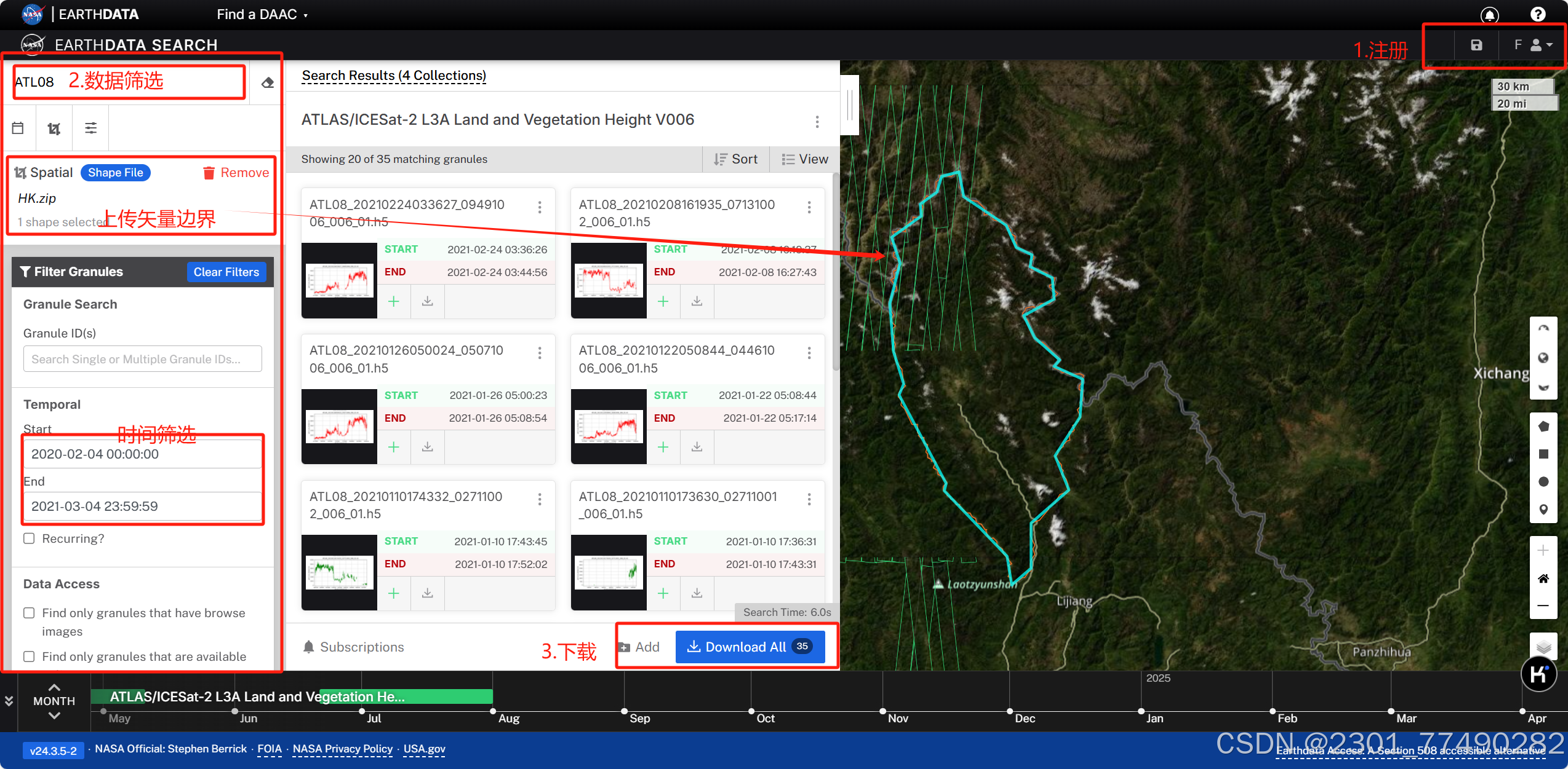
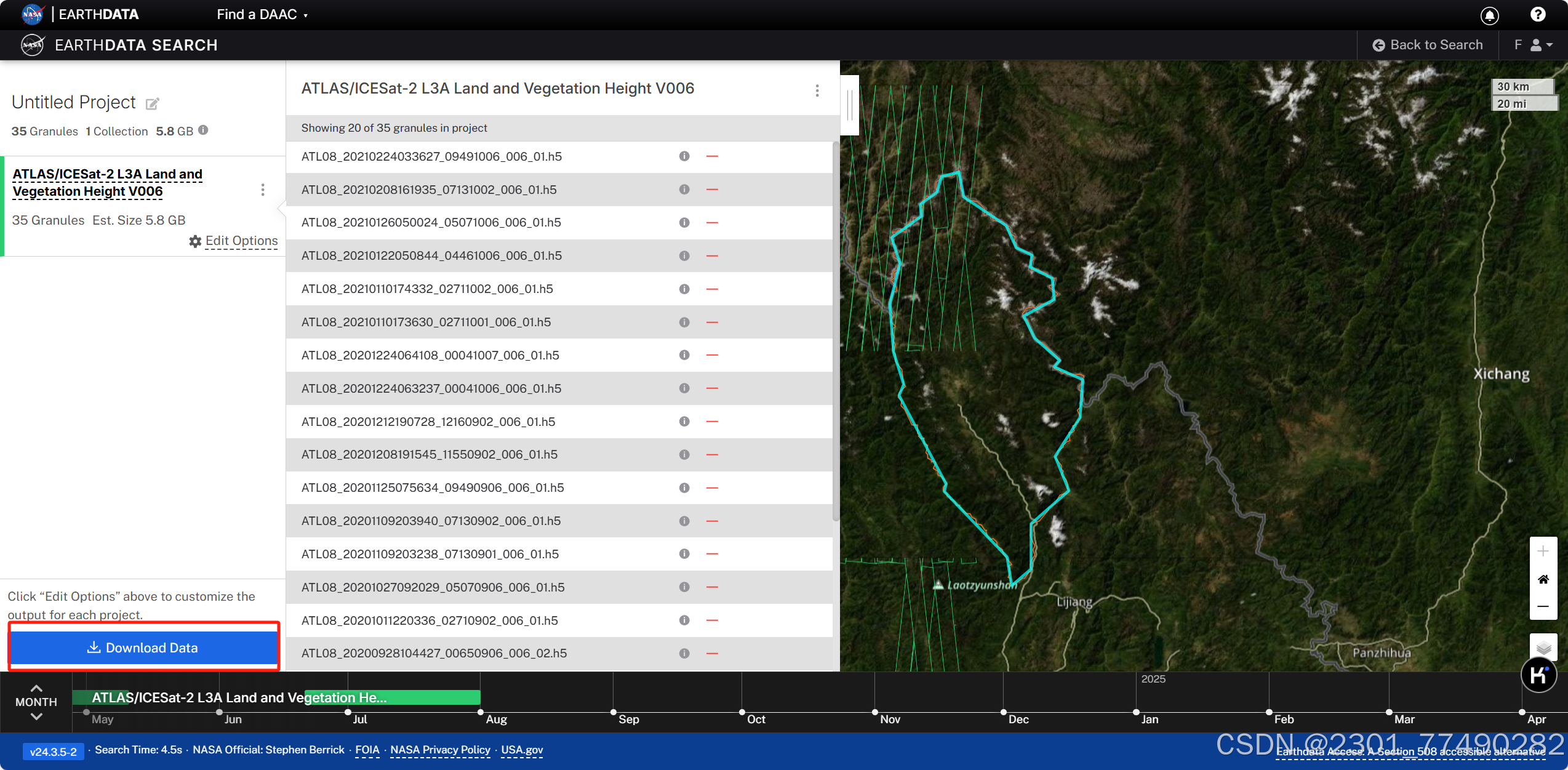
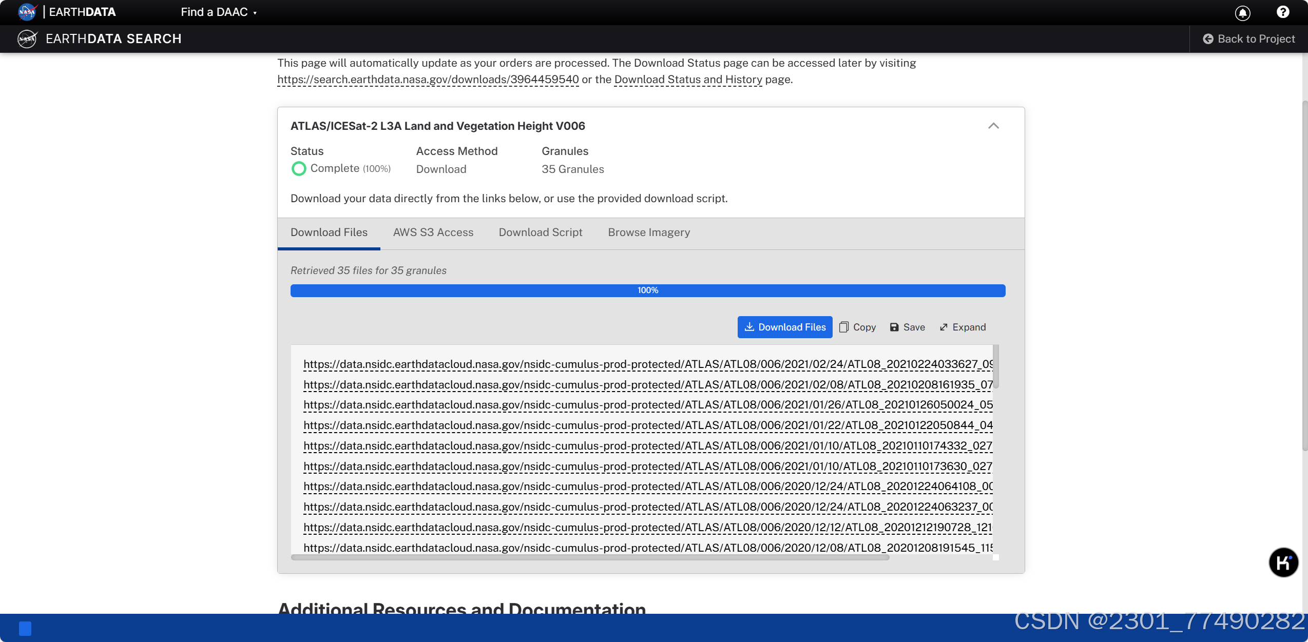
数据下载
(批量下载可查看上一篇博文:如何批量下载ICESat-2数据(无需代码)-CSDN博客)
数据下载地址:
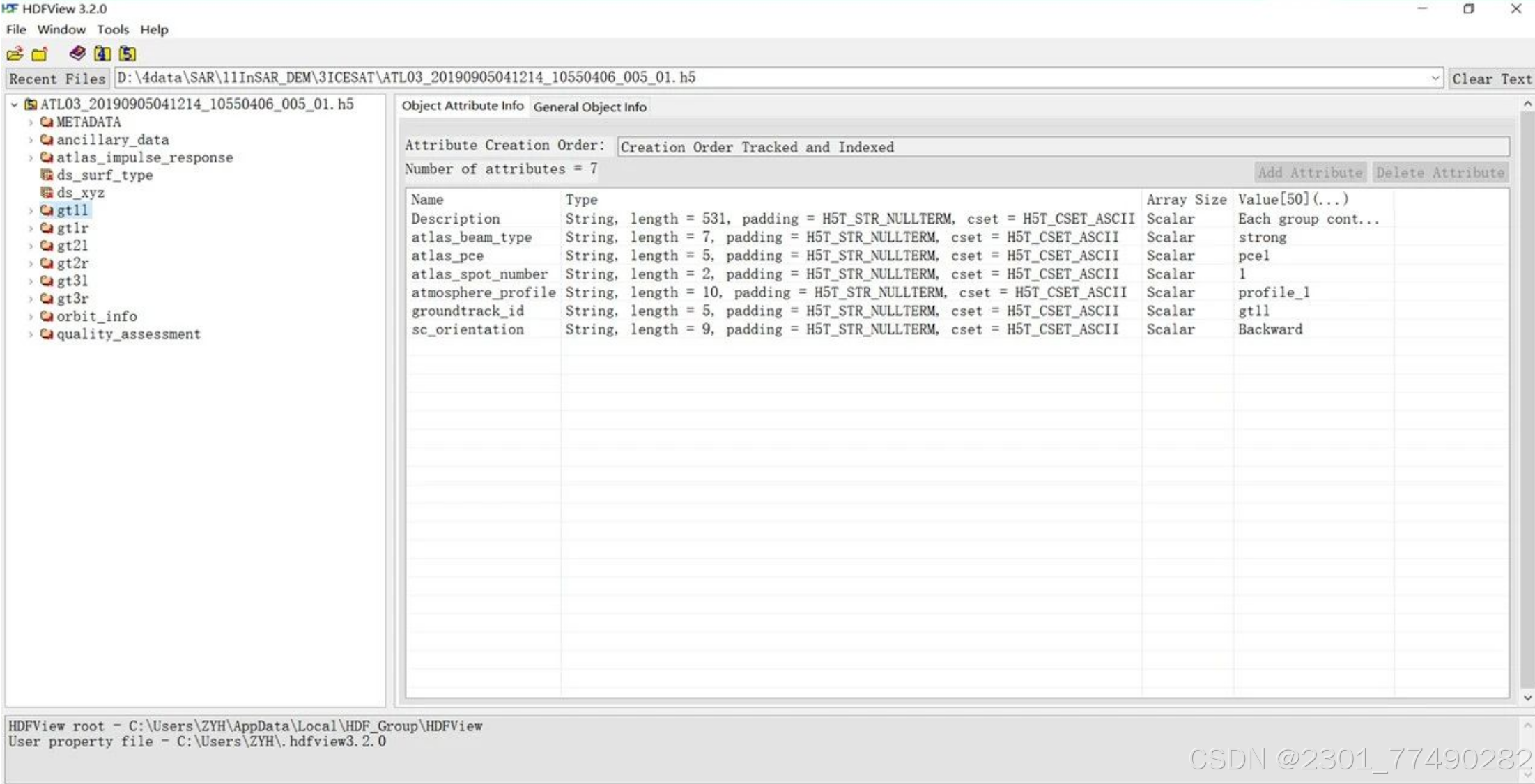
数据查看
ICEsat-2下载的数据是以HD5.格式存储的,可以下载HDFView进行数据查看
下载链接:https://portal.hdfgroup.org/display/support/HDFView+3.2.0#files
数据处理
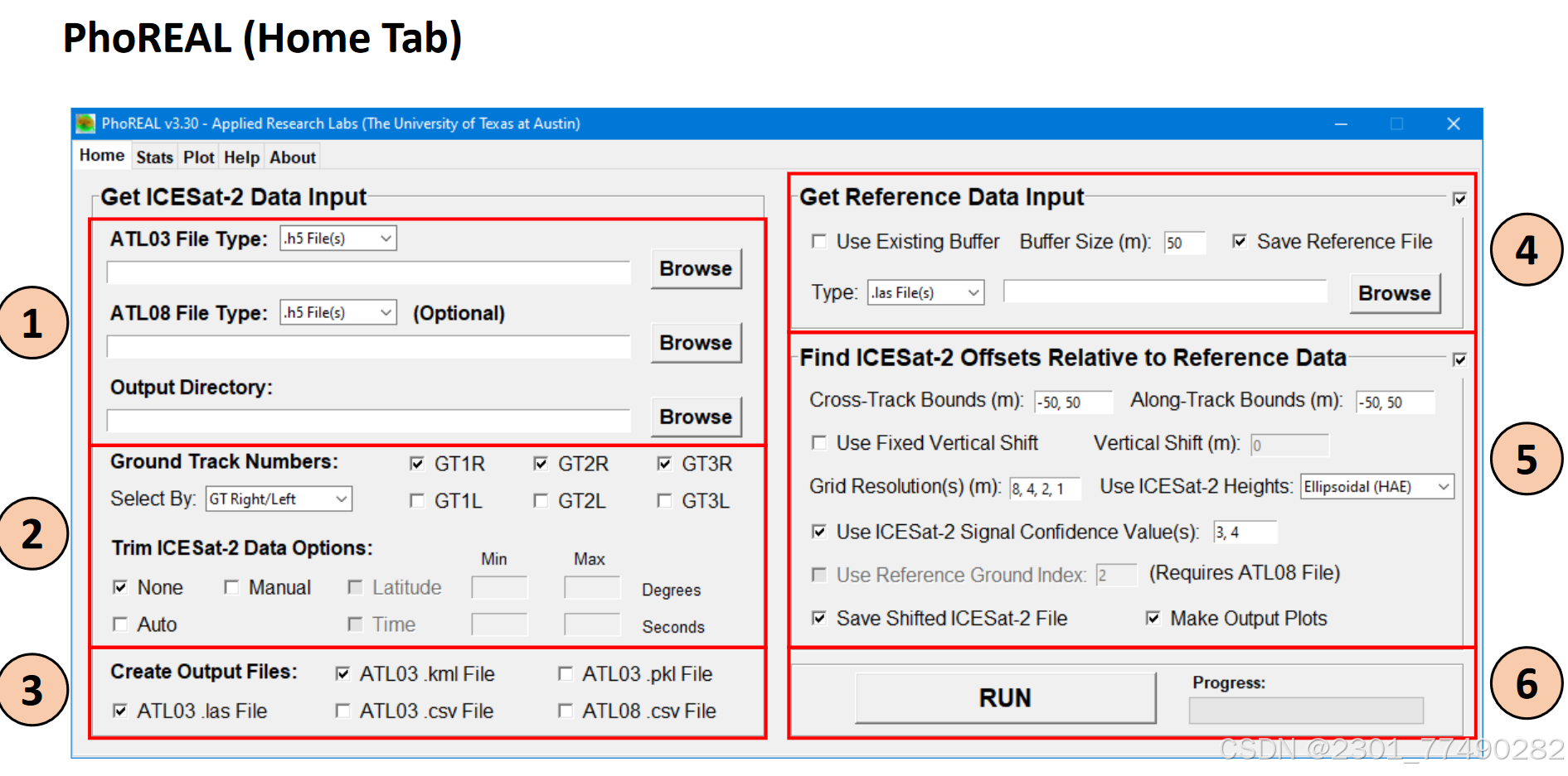
下载PhoREAL(粗处理)
Phoreal(Photon Research and Engineering Synery Sycorage)是一个地理空间分析工具箱,允许用户读取,处理,分析和制图以及输出ICESAT-2 ATL03和ATL08数据。
项目地址:https://gitcode.com/open-source-toolkit/8f473
数据处理页面:
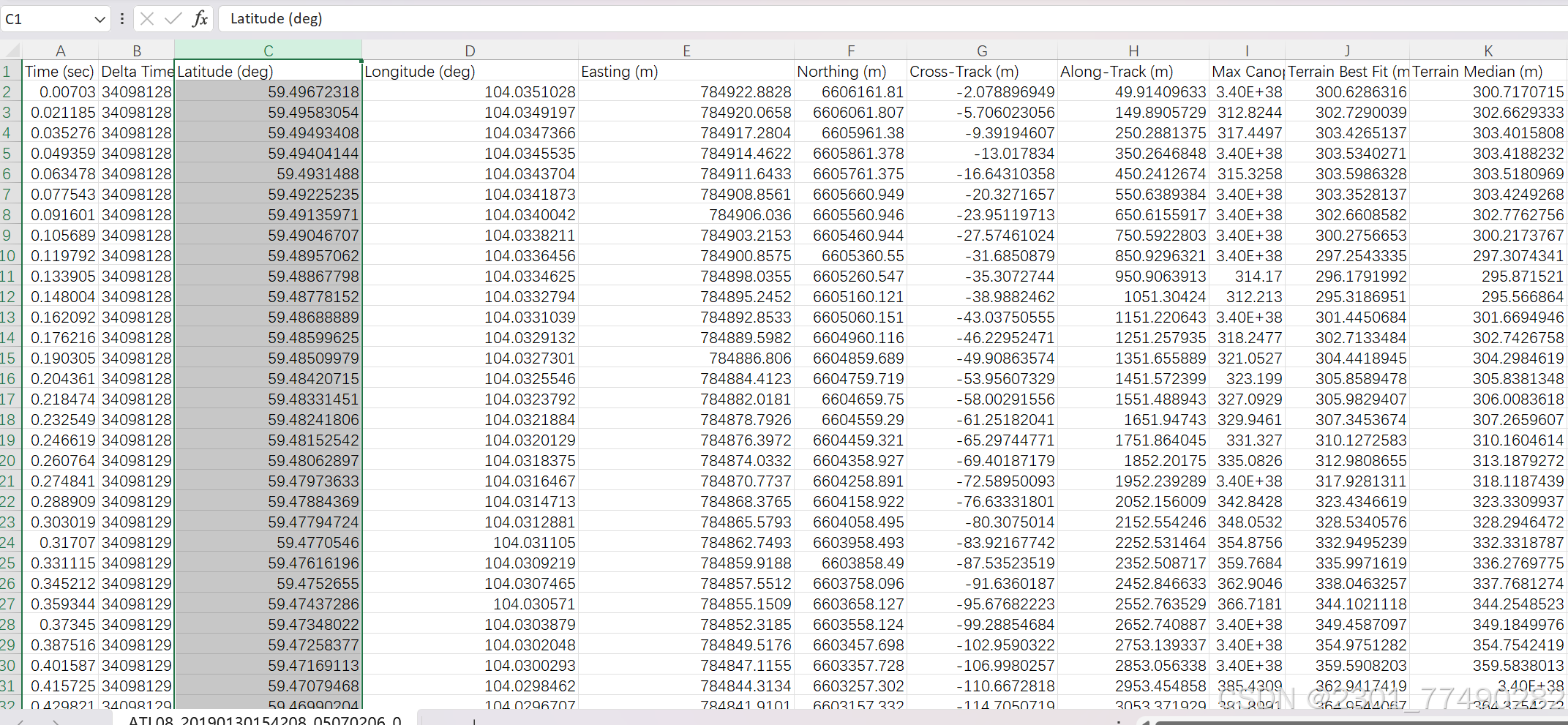
PhoREAL可导出激光点高程冠层高及坐标等信息
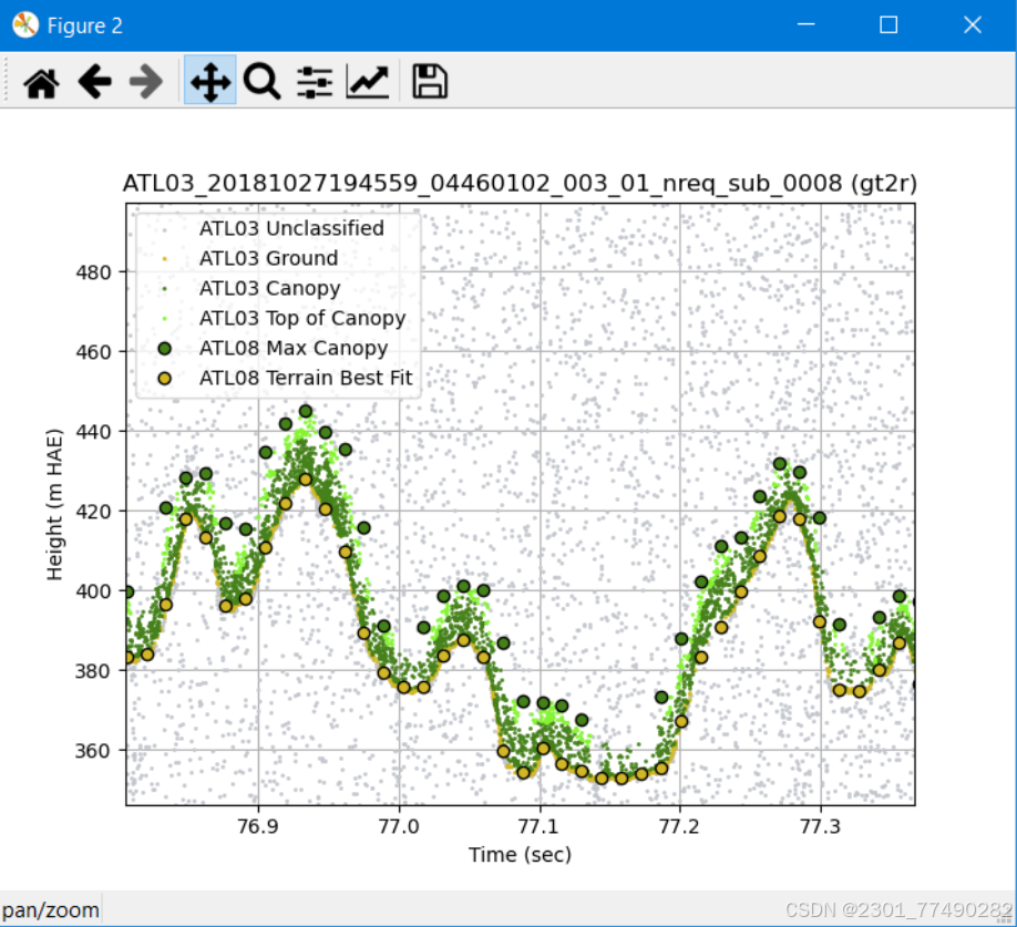
数据制图页面:
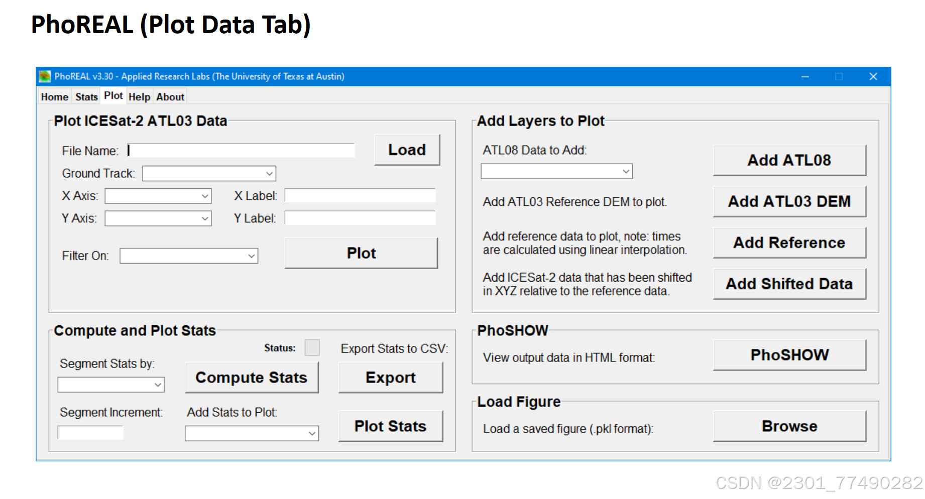
导入ARCgis进行后续分析
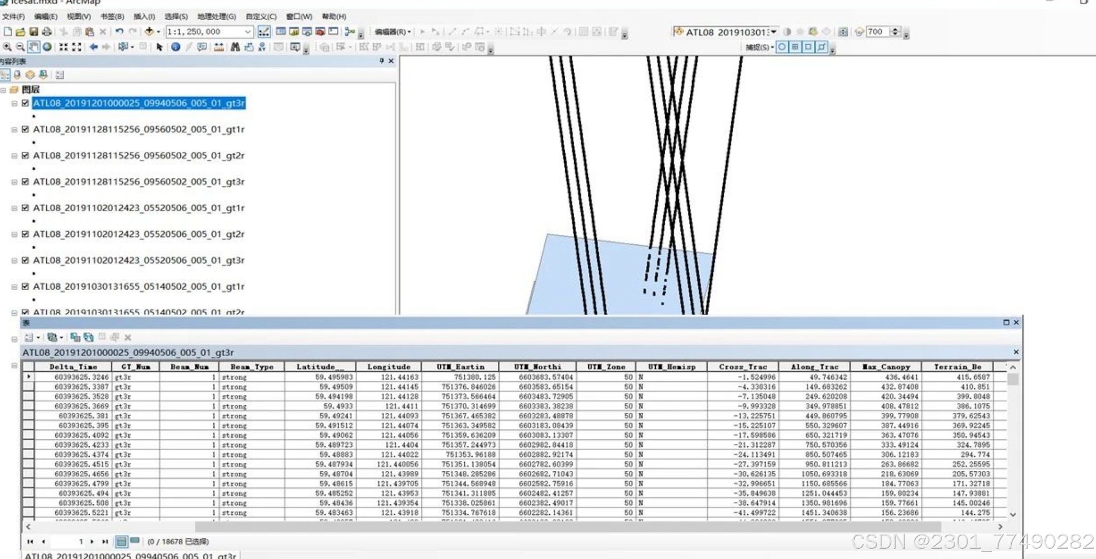
精细化处理ICEsat-2 ATL08和ATL03 数据
在ICESat-2数据处理中,ATL03和ATL08数据产品都可能需要去噪处理,但它们的目的和处理方式有所不同。
-
ATL03数据产品:
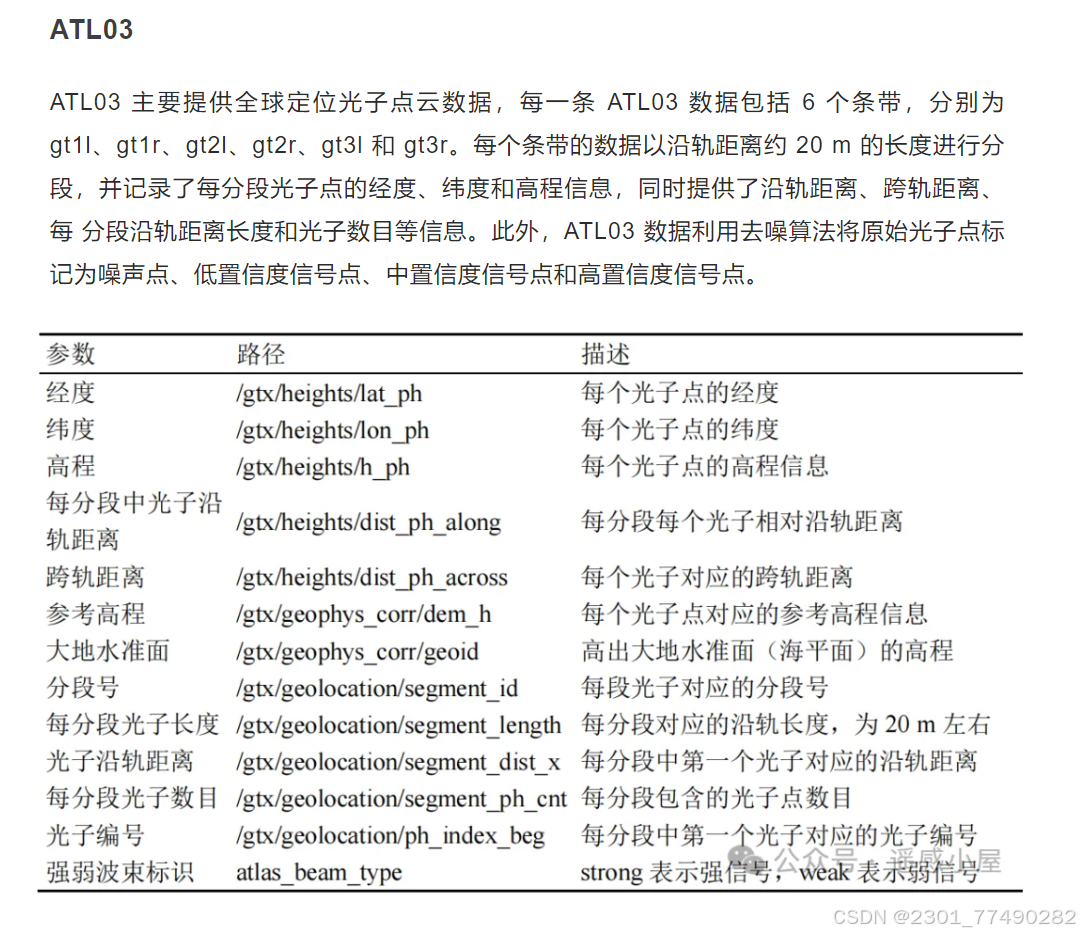
- ATL03提供了每个接收到的光子的精确纬度、经度和高程,并且光子被分类为信号与背景,以及地表类型(如陆地冰、海冰、陆地、海洋)。
- 由于ATL03数据包含了所有的光子信息,包括噪声光子和信号光子,因此在使用这些数据进行地形、冰层或植被分析之前,通常需要进行去噪处理以分离出有用的信号光子。
- 去噪处理的目的是去除大气散射、云层和其他非地面反射的噪声光子,从而提取出代表地表的信号光子。
-
ATL08数据产品:
- ATL08数据产品已经通过官方算法对经过初步噪声剔除的ATL03数据进行了进一步信号光子分类和噪声滤除。
- ATL08数据提供了冠层高度、冠层覆盖率、表面坡度和粗糙度,以及表观反射率等信息,这些数据已经是基于去噪后的光子数据得到的。
- 因此,ATL08数据产品通常不需要用户再次进行去噪处理,除非有特殊的分析需求或要进一步优化数据质量。
在实际应用中,是否需要进行去噪处理取决于分析目标和数据的质量。如果目的是进行高精度的地形或植被分析,那么对ATL03数据进行去噪和分类是必要的。而去噪的方法有多种,包括基于统计的方法、基于密度的方法(如DBSCAN或OPTICS算法),或者使用专门的软件工具如PhoREAL进行处理。
总结来说,ATL03数据通常需要去噪以提取有用的地表信息,而ATL08数据产品已经包含了去噪后的光子数据,一般不需要再次去噪,除非有特殊的分析需求。
去噪算法
算法一(基于统计的去噪和基于半径的去噪)
import pandas as pd
import open3d as o3d
import numpy as np
import matplotlib.pyplot as plt

# 【提示】噪声和数据的时间也有关系,最好下载晚上的数据,白天的数据噪声多且数据量大(因为都是噪点)
# 该代码在处理后的新csv会仅存去噪后的点云,噪点被删去

inputCSVpath = "E:/ICEsat2/ATL03_L08-6/outputtest/L03_55.csv"
outputCSVpath = "E:/ICEsat2/ATL03_L08-6/outputtest/L03_55_inliers_radius.csv"

def statistical_outlier_removal(pcd, neighbors=20, ratio=2.0):
    cl, ind = pcd.remove_statistical_outlier(nb_neighbors=neighbors, std_ratio=ratio)
    inlier_cloud = pcd.select_by_index(ind)
    outlier_cloud = pcd.select_by_index(ind, invert=True)
    return ind, outlier_cloud, inlier_cloud

def radius_outlier_removal(pcd, nb_points=16, radius=10):
    cl, ind = pcd.remove_radius_outlier(nb_points=nb_points, radius=radius)
    inlier_cloud = pcd.select_by_index(ind)
    outlier_cloud = pcd.select_by_index(ind, invert=True)
    return ind, outlier_cloud, inlier_cloud

# 读取ATL03 CSV数据
atlo3_data = pd.read_csv(inputCSVpath)

# 将数据转换为点云
point_cloud = o3d.geometry.PointCloud()
#这里横纵坐标也可以变
point_cloud.points = o3d.utility.Vector3dVector(atlo3_data[['dist_ph_along','dist_ph_across', 'h_ph']].values)


# 【基于半径阈值的方法,后面还有基于统计的方法】
# 对点云进行半径异常点移除
inlier_indices_radius, outlier_cloud_radius, inlier_cloud_radius = radius_outlier_removal(point_cloud)

# 提取半径异常点移除后的内点对应的行
inlier_data_radius = atlo3_data.iloc[inlier_indices_radius]

# 将内点数据保存为新的CSV文件
inlier_data_radius.to_csv(outputCSVpath, index=False)

# 可视化原始点云和去噪后的点云
# 转换为numpy数组以便可视化
outlier_points_radius = np.asarray(outlier_cloud_radius.points)
inlier_points_radius = np.asarray(inlier_cloud_radius.points)

plt.figure(figsize=(10, 8))

# 绘制半径异常点移除结果
plt.scatter(outlier_points_radius[:, 0], outlier_points_radius[:, 2], c='gray', label='Radius Outliers', s=0.5)
plt.scatter(inlier_points_radius[:, 0], inlier_points_radius[:, 2], c='red', label='Radius Inliers', s=1)

# 设置图例
plt.legend()

# 设置坐标轴标签
plt.xlabel('Distance along the track(m)')
plt.ylabel('height(m)')

# 显示图形
plt.show()


# 【基于统计的方法,我感觉在噪声多的时候没有基于半径的方法好用】
# 对点云进行统计异常点移除
# inlier_indices_statistical, outlier_cloud_statistical, inlier_cloud_statistical = statistical_outlier_removal(point_cloud)
# 提取统计异常点移除后的内点对应的行
# inlier_data_statistical = atlo3_data.iloc[inlier_indices_statistical]
# 转换为numpy数组以便可视化
# outlier_points_statistical = np.asarray(outlier_cloud_statistical.points)
# inlier_points_statistical = np.asarray(inlier_cloud_statistical.points)
# 将内点数据保存为新的CSV文件
# inlier_points_statistical.to_csv("D:/ICEsat2/ATL03_L08-6/L03_55_inliers_statistical.csv", index=False)
# plt.figure(figsize=(10, 8))
# 绘制统计异常点移除结果
# plt.scatter(outlier_points_statistical[:, 0], outlier_points_statistical[:, 2], c='red', label='Statistical Outliers', s=1)
# plt.scatter(inlier_points_statistical[:, 0], inlier_points_statistical[:, 2], c='gray', label='Statistical Inliers', s=1)
# 设置图例
# plt.legend()
#
# # 设置坐标轴标签
# plt.xlabel('Distance along the track(m)')
# plt.ylabel('height(m)')
#
# # 显示图形
# plt.show()算法二(基于K邻域平均距离)
import tkinter as tk
from tkinter import filedialog
import pandas as pd
import numpy as np
import matplotlib.pyplot as plt
from scipy.spatial import KDTree

# 打开文件选择弹窗并选择文件
def open_file_dialog():
    root = tk.Tk()
    root.withdraw()  # 隐藏主窗口
    file_path = filedialog.askopenfilename(title="Select ICESat-2 CSV File", filetypes=[("CSV files", "*.csv")])
    return file_path

# 计算K邻域内的平均距离平方
def calculate_dist_ave(along_track, height, K=5):
    dist_ave = np.zeros(len(along_track))
    for i in range(len(along_track)):
        neighbors_idx = np.arange(max(0, i - K // 2), min(len(along_track), i + K // 2 + 1))
        neighbors = np.sqrt(
            (along_track[i] - along_track[neighbors_idx]) ** 2 + (height[i] - height[neighbors_idx]) ** 2)
        dist_ave[i] = np.mean(neighbors)
    return dist_ave

# 去噪处理函数
def remove_noise(df, avg_distances, threshold=1):
    # 根据平均距离和阈值判断噪声
    signal_mask = avg_distances < threshold
    df_valid = df[signal_mask]  # 有效信号
    df_noise = df[~signal_mask]  # 噪声点
    valid_points = df_valid.index  # 有效点的索引
    return df_valid, df_noise, avg_distances, valid_points

# 去噪处理
def denoise_data(df, along_track, height, threshold=2, K=5):
    avg_distances = calculate_dist_ave(along_track, height, K)
    df_valid, df_noise, avg_distances, valid_points = remove_noise(df, avg_distances, threshold)
    return df_valid, df_noise, avg_distances

# 主函数
def main():
    # 打开文件
    file_path = open_file_dialog()

    # 读取CSV文件
    data = pd.read_csv(file_path)
    along_track = data['Along-Track (m)'].values
    height = data['Height (m HAE)'].values

    # 去噪处理
    df_valid, df_noise, avg_distances = denoise_data(data, along_track, height)

    # 画图
    plt.figure(figsize=(12, 8))
    # 原始数据图
    plt.subplot(3, 1, 1)
    plt.scatter(along_track, height, s=0.01, c='blue', label='Original Data')
    plt.xlabel('Along-Track (m)')
    plt.ylabel('Height (m HAE)')
    plt.title('Original ICESat-2 Data')
    plt.legend()

    # 平均距离图 - 使用颜色条来表示 Average Distance
    plt.subplot(3, 1, 2)
    # 使用scatter, c=avg_distances 表示用颜色条映射平均距离的值,cmap是颜色映射
    sc = plt.scatter(along_track, avg_distances, c=avg_distances, cmap='magma', s=0.1, label='Average Distance')
    # 添加颜色条,表示平均距离的数值
    cbar = plt.colorbar(sc)
    cbar.set_label('Average Distance')
    # 坐标轴和标题
    plt.xlabel('Along-Track (m)')
    plt.ylabel('Average Distance')
    plt.title('Average Distance of K Neighbors')
    # 添加图例
    plt.legend()

    '''
    # 平均距离图
    plt.subplot(3, 1, 2)
    plt.plot(along_track, avg_distances, c='orange', label='Average Distance (K Neighbors)')
    plt.xlabel('Along-Track (m)')
    plt.ylabel('Average Distance')
    plt.title('Average Distance of K Neighbors')
    plt.legend()
    '''

    # 去噪后数据图
    plt.subplot(3, 1, 3)
    plt.scatter(df_valid['Along-Track (m)'], df_valid['Height (m HAE)'], s=1, c='red', label='Denoised Data')
    plt.xlabel('Along-Track (m)')
    plt.ylabel('Height (m HAE)')
    plt.title('Denoised ICESat-2 Data')
    plt.legend()

    # 显示图形
    plt.tight_layout()
    plt.show()

if __name__ == '__main__':
    main()
算法三(基于密度聚类的算法)
import warnings
warnings.filterwarnings('ignore')

import pandas as pd
import matplotlib.pyplot as plt
from sklearn.cluster import DBSCAN
from sklearn.preprocessing import StandardScaler
from sklearn.metrics import silhouette_score

# 输入 csv 文件
csv_path = r"D:\7Miscellaneous Notes\xainggelila\ATL03_20190130154208_05070206_006_02_gt1r.csv"

# 读取数据
d1 = pd.read_csv(csv_path)

# 选择沿轨距离和高度信息
req_col = ["Height (m MSL)", "Along-Track (m)"]

# 查看所选数据
print(d1[req_col].head())

# 使用 StandardScaler 标准化功能
z = StandardScaler()
d1[["Height (m MSL)", "Along-Track (m)"]] = z.fit_transform(d1[["Height (m MSL)", "Along-Track (m)"]])

# 标准化特征
print(d1[["Height (m MSL)", "Along-Track (m)"]].head())

# 画图
plt.scatter(d1["Along-Track (m)"], d1["Height (m MSL)"])
plt.ylabel("Photon Height")
plt.xlabel("Along-Track (m)")
plt.rcParams['font.sans-serif'] = ['STSong']
plt.rcParams['axes.unicode_minus'] = False
plt.title("原始数据")
plt.show()

# 执行 DBSCAN 去噪
db1 = DBSCAN(eps=0.2, min_samples=15).fit(d1[req_col])

# 更新 DataFrame 中的标签
d1["assignments"] = db1.labels_
labsList = ["Noise"] + ["Cluster" + str(i) for i in range(1, len(set(db1.labels_)))]

# 结果图
plt.scatter(d1["Along-Track (m)"], d1["Height (m MSL)"], s=5, c=db1.labels_)
plt.ylabel("Photon Height")
plt.xlabel("Along-Track (m)")
plt.rcParams['font.sans-serif'] = ['STSong']
plt.rcParams['axes.unicode_minus'] = False
plt.title("DBSCAN 去噪")
plt.colorbar(label="聚类分配")
plt.legend(labsList)
plt.show()

# 选择用于轮廓分数计算的聚类数据点
d1_clustered = d1.loc[d1["assignments"] >= 0]

# 检查集群数据中是否至少有两个唯一标签
unique_labels = d1_clustered["assignments"].unique()
if len(unique_labels) < 2:
    print("用于轮廓分数计算的标签数量不足.")
else:
    # 计算聚类数据点的轮廓分数
    silhouette = silhouette_score(d1_clustered[["Along-Track (m)", "Height (m MSL)"]], d1_clustered["assignments"])
    print("群集数据点的轮廓分数:", silhouette)

# 计算数据集的总体轮廓得分
silhouette_overall = silhouette_score(d1[["Along-Track (m)", "Height (m MSL)"]], d1["assignments"])
print("整体轮廓得分:", silhouette_overall)

# 将带有聚类分配的 DataFrame 保存为新的 CSV 文件
d1.to_csv('clustered_data.csv', index=False)
分类算法
1.使用专门的软件工具如PhoREAL进行处理
2.CSF 算法
import pandas as pd  # pandas是用于数据处理和分析的强大工具。
import numpy as np  # numpy用于数值计算和数组操作
import matplotlib.pyplot as plt   # 导入matplotlib的pyplot模块,并将其别名为plt。用于绘制图形和可视化数据。
import CSF as CSFF  # 算法
from tkinter import Tk, filedialog  # 从tkinter库中导入Tk类和filedialog模块。用于创建图形用户界面和选择文件对话框。
from tqdm import tqdm  # 用于显示进度条
import time  # 导入时间模块,用于获取时间信息。
#  from scipy import interpolate
#  from scipy.interpolate import interp1d


def select_file():
    Tk().withdraw()
    file_path = filedialog.askopenfilename()
    return file_path


def save_file():
    Tk().withdraw()
    file_path = filedialog.asksaveasfilename(defaultextension=".csv")
    return file_path


def segment_filter(file=None, outfile=None, segment_calculation=1):
    if file is None:
        file = select_file()
    if outfile is None:
        outfile = save_file()

    data = pd.read_csv(file)

    if 'Terrain Median (m)' in data.columns and 'Height (m HAE)' not in data.columns:
        data.rename(columns={'Terrain Median (m)': 'Height (m HAE)'}, inplace=True)
        print("重命名后的列名:", data.columns)

    x = data["Along-Track (m)"]
    y = data["Cross-Track (m)"]
    z = data["Height (m HAE)"]

    segment_length = 30
    num_segments = len(data) // segment_length
    segments = [data.iloc[i*segment_length:(i+1)*segment_length] for i in range(num_segments)]

    filtered_segments = []
    csf = CSFF.CSF()
    csf.params.bSloopSmooth = True
    csf.params.cloth_resolution = 5
    csf.params.rigidness = 2
    csf.params.time_step = 1
    csf.params.class_threshold = 4
    csf.params.interations = 1000

    start_time = time.time()
    if segment_calculation == 1:
        for segment in tqdm(segments, desc="开始滤波", unit="segment"):
            latitude = segment["Along-Track (m)"]
            longitude = segment["Cross-Track (m)"]
            height = segment["Height (m HAE)"]
            print("-------点云分类开始--------")
            xyz = np.vstack((longitude, latitude, height))
            csf.setPointCloud(xyz)
            ground = CSFF.VecInt()
            non_ground = CSFF.VecInt()
            csf.do_filtering(ground, non_ground)
            segment_indices = set(segment.index)
            valid_indices = list(segment_indices.intersection(ground))
            ground_data = segment.loc[valid_indices]
            filtered_segments.append(ground_data)
            tqdm.write(f"已处理 {len(filtered_segments)} / {len(segments)} 个 segment")
    else:
        latitude = data["Along-Track (m)"]
        longitude = data["Cross-Track (m)"]
        height = data["Height (m HAE)"]
        print("-------点云分类开始--------")
        xyz = np.vstack((longitude, latitude, height))
        csf.setPointCloud(xyz)
        ground = CSFF.VecInt()
        non_ground = CSFF.VecInt()
        csf.do_filtering(ground, non_ground)
        segment_indices = set(data.index)
        valid_indices = list(segment_indices.intersection(ground))
        ground_data = data.loc[valid_indices]
        filtered_segments.append(ground_data)
        tqdm.write(f"已处理完整个点云数据")

    end_time = time.time()
    processing_time = end_time - start_time

    filtered_data = pd.concat(filtered_segments)
    filtered_data.to_csv(outfile, index=False)

    print("处理完成!")
    print("处理时间:{:.2f}秒".format(processing_time))

    return data, filtered_data


def plot_points(data, filtered_data):
    # 进行地面点加密
    # 使用三次样条曲线拟合地面线


    # 绘制原始数据的散点图
    plt.figure(figsize=(10, 5))
    plt.subplot(1, 2, 1)
    plt.scatter(data["Along-Track (m)"], data["Cross-Track (m)"], c=data["Height (m HAE)"], cmap='terrain')
    plt.title('Original Data')
    plt.xlabel('Along-Track (m)')
    plt.ylabel('Cross-Track (m)')
    plt.colorbar(label='Height (m HAE)')

    # 绘制滤波后数据的散点图
    plt.subplot(1, 2, 2)
    plt.scatter(filtered_data["Along-Track (m)"], filtered_data["Cross-Track (m)"], c=filtered_data["Height (m HAE)"], cmap='terrain')
    plt.title('Filtered Data')
    plt.xlabel('Along-Track (m)')
    plt.ylabel('Cross-Track (m)')
    plt.colorbar(label='Height (m HAE)')

    plt.tight_layout()
    plt.show()

if __name__ == "__main__":
    data, filtered_data = segment_filter(segment_calculation=0)
    plot_points(data, filtered_data)
数据关联
前言
ICESat-2中的ATL03数据再进行运用时一般需要进行去噪分类等流程,最后得到的结果好坏主要取决于处理算法的优劣。其实,ICESat-2的ATL08 数据产品就已经通过官方算法对经过初步噪声剔除的 ATL03 数据进行了进一步信号光子分类和噪声滤除,在一定程度上省去了对ATL03数据的繁琐处理。但是尽管 ATL08 数据产品提供了每一个光子的类别与高度信息,但是并没有提供光子点相应的位置信息,这在实际应用中受到限制。
所以,通过Python实现ICESat-2的ATL03 与 ATL08 数据关联,从而得到每个光子位置所对应的位置等信息,为后续的森林高度反演、生物量估计等研究提供支持。
ATL03数据
ATL08
ATL08 是陆地植被高度产品,它是通过对 ATL03 产品进一步去噪获取信号点,然后将信号点分类为地面光子点、植被冠层顶部光子点和冠层光子点,并提取沿轨距离每 100 m 分段对应的地面高程和植被高度信息。其中地面高程信息包括最佳拟合地面高程、最大地面高程、平均地面高程、地面高程中位数、最小地面高程等。森林高度包括最大森林高度、平均森林高度、森林高度中位数、最小森林高度和森林高度百分位数(25%,50%,60%,70%,75%,80%,85%,90%,95%, 98%森林高度)等。此外 ATL08 产品提供了每 100 m 分段对应的信噪比、坡度、云量、地面高程不确定性和森林高度不确定性信息等。

ATL03 沿轨距离每隔 20m 划分为一个区段,ATL08 沿轨距离每隔 100m 划分为一个区 段。其中,100m 分段是由一共 5 段 20m 分段组成,20m 分段在 ATL03 和 ATL08 数据中由 segment id 连接。
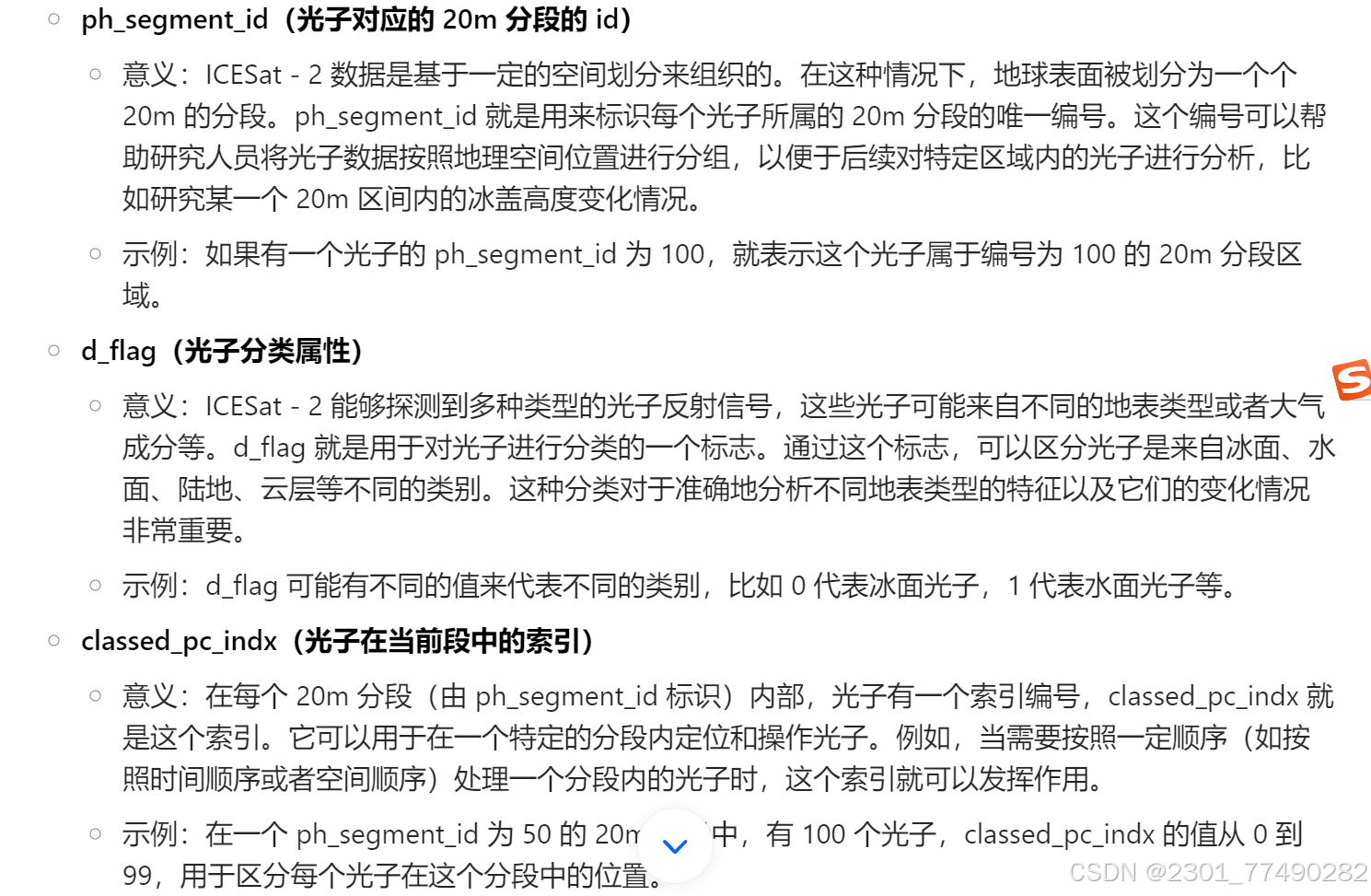
”ATL08: ph_segment_id (光子对应的20m分段的id)、d_flag(光子分类属性)、classed_pc_indx(光子在当前段中的索引)
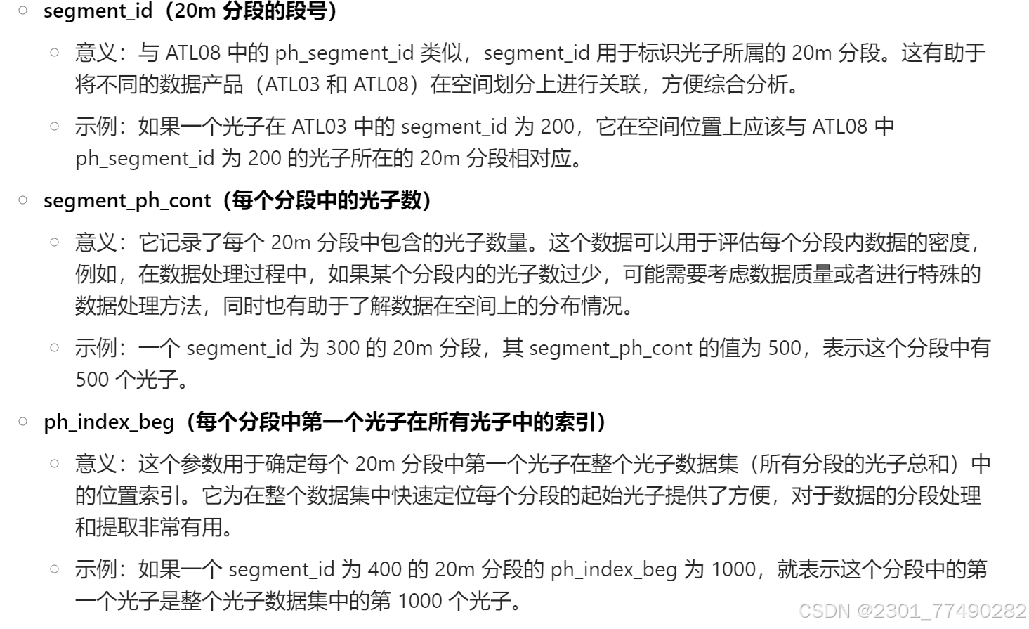
ATL03:h_ph(光子高程)、lat_ph(光子纬度)、lon_ph(光子经度)、segment_id(20m分段的段号)、segment_ph_cont(每个分段中的光子数)、ph_index_beg(每个分段中第一个光子在所有光子中的索引)
看到用到的数据其实大概就已经能猜到两个文件的对应关系了,它是通过20m分段来进行对应的。那么我们要实现每个分段中光子的对应就需要按以下3步来进行:
找到ATL08中数据在ATL03中的分段。
按照ATL08分段中每个光子的索引对应查找其在ATL03所有光子中的索引。
按照查找到的ATL03索引找到对应的经纬度和高程坐标,然后将其与ATL08中的属性组合起来。”
原文链接:https://blog.csdn.net/qq_29949039/article/details/132591852
一、整体流程概述
这个过程主要是通过利用 ATL08 数据中的特定信息(如 20m 分段 id 和光子在当前段中的索引),结合 ATL03 数据中的相关参数,来确定一个光子在整个数据集里的位置索引,进而找到该光子对应的经纬度坐标和高程等信息。如果需要,还可以将经纬度信息投影到投影坐标系以满足特定的分析需求。
二、步骤详解及示例
-
拿到 ATL08 一个光子
- 假设我们拿到的这个光子在 ATL08 数据中的 ph_segment_id 为 123,classed_pc_indx(光子在当前段中的索引)为 15。
-
用该光子的 20m 分段 id 减去 ATL03 数据中第一个 20m 分段 id,得到这个光子对应于所有 20m 分段的索引 index
- 假设 ATL03 数据中第一个 20m 分段的 segment_id 为 100。
- 那么这个光子对应于所有 20m 分段的索引 index = 123 - 100 = 23。
-
根据该 index 得到这个分段中第一个光子在所有光子数据中的索引 idx_all
- 在 ATL03 数据中,每个 20m 分段都有一个 ph_index_beg 参数,表示该分段中第一个光子在所有光子中的索引。
- 假设对应 index = 23 的这个分段,其 ph_index_beg 的值为 5000。
- 那么 idx_all = 5000。
-
根据 idx_all 加上 ATL08 光子在当前段内是第几个光子的索引,得到该光子在所有光子中的索引 idx
- 已知 ATL08 中该光子在当前段中的索引 classed_pc_indx 为 15。
- 所以该光子在所有光子中的索引 idx = idx_all + classed_pc_indx = 5000 + 15 = 5015。
-
根据 idx 找到对应的经纬度坐标、高程等信息
- 在 ATL03 数据中,根据索引 idx = 5015,可以找到该光子对应的 h_ph(光子高程)、lat_ph(光子纬度)、lon_ph(光子经度)等信息。
- 假设这些信息分别为:h_ph = 1200 米,lat_ph = 45°N,lon_ph = 80°E。
-
如果需要的话将经纬度信息投影到投影坐标系
- 例如,如果需要在平面地图上进行分析,可以将经纬度(45°N,80°E)投影到特定的投影坐标系中,如墨卡托投影坐标系,得到对应的平面坐标值。
通过以上步骤,就可以从 ATL08 和 ATL03 数据中找到特定光子的坐标数据及高程信息。
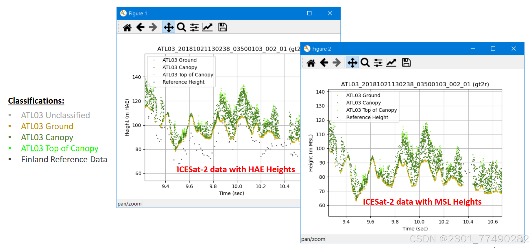
ATL08 数据对经过初步噪声剔除的 ATL03 数据进行进一步信号光子 分类和噪声滤除,主要操作步骤包括地面曲线拟合和植被表面曲线拟合,被用于地面曲线 拟合的光子标记为地面光子(Groud),被用于植被表面曲线拟合的光子标记为冠层顶部光子 (Top of canopy),介于两条曲线之间的光子被标记为冠层(Canopy),其余光子被标记为噪声 (Noise)。如图所示,为 ATL03 和 ATL08 数据匹配示意图。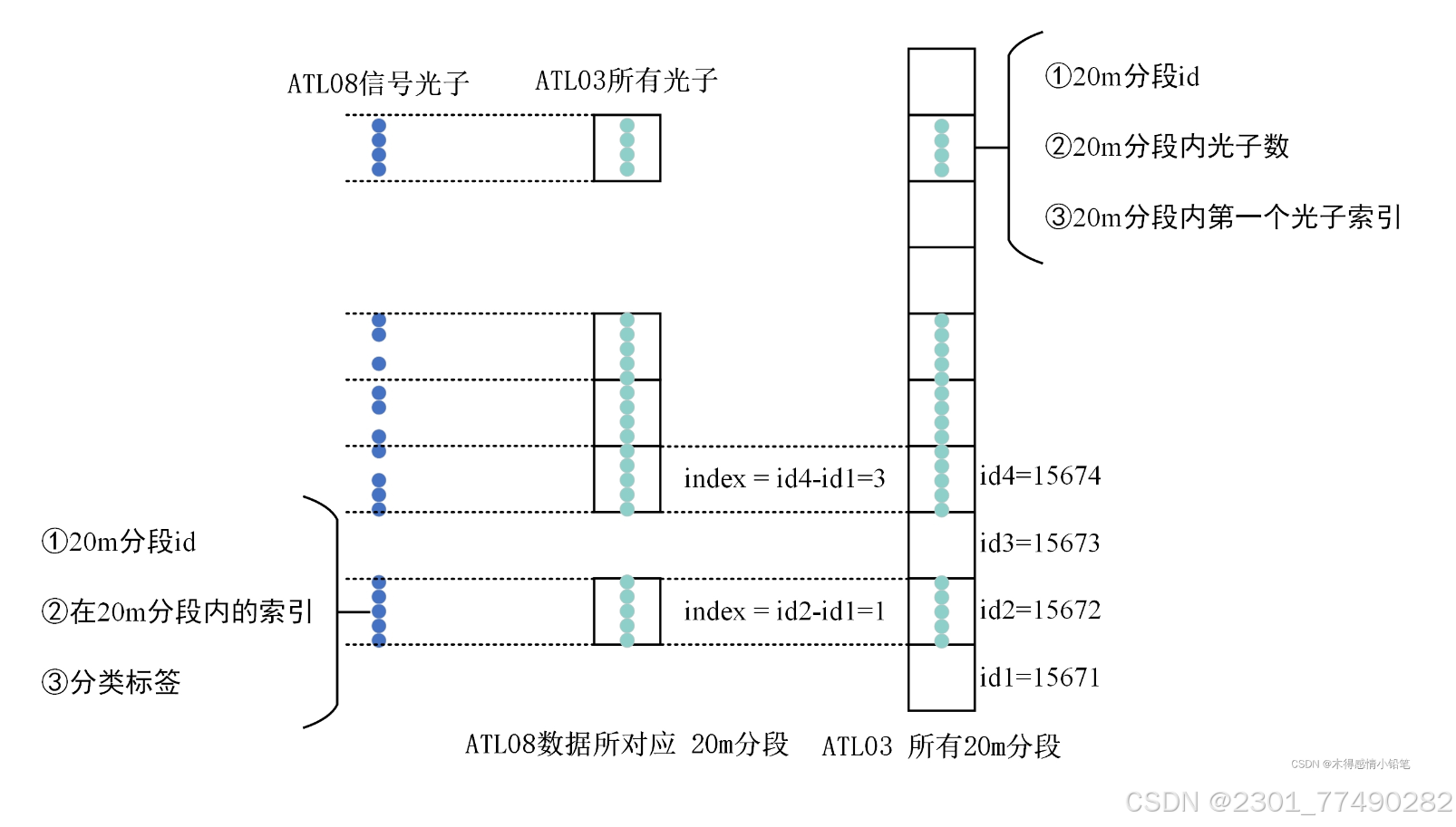
ATL03 与 ATL08 数据关联
"""
关联 ATL08 与 ATL03 数据产品,实现以下步骤:
1. 遍历 ATL08 和 ATL03 数据产品的每个光子。
2. 利用光子区间号匹配(ph_segment_id=segment_id),找到两组数据的相同区间。
3. 逐个匹配每个光子,通过 ATL03 数据的起始光子序号与 ATL08 数据的相对光子序号相加(classed_pc_indx+ph_index_beg-1),将 ATL08 的每个光子对应在 ATL03 数据产品中。
"""

import h5py
import numpy as np
from tqdm import tqdm
import time
import pandas as pd
import matplotlib.pyplot as plt


class ATLDataLoader:
    def __init__(self, atl03_path, atl08_path, gtx):
        """
        初始化类,设置数据文件路径和光束名称,并加载数据。

        :param atl03_path: ATL03 文件路径。
        :param atl08_path: ATL08 文件路径。
        :param gtx: 光束名称。
        """
        self.atl03Path = atl03_path
        self.atl08Path = atl08_path
        self.gtx = gtx
        self.load()

    def load(self):
        """
        加载 ATL03 和 ATL08 数据,进行数据关联。
        """
        # 读取 ATL03 分段数据
        with h5py.File(self.atl03Path, 'r') as f:
            self.atl03_lat = np.array(f[self.gtx + '/heights/lat_ph'][:])
            self.atl03_lon = np.array(f[self.gtx + '/heights/lon_ph'][:])
            self.atl03_ph_index_beg = np.array(f[self.gtx + '/geolocation/ph_index_beg'][:])
            self.atl03_segment_id = np.array(f[self.gtx + '/geolocation/segment_id'][:])
            self.atl03_heights = np.array(f[self.gtx + '/heights/h_ph'][:])
            self.atl03_conf = np.array(f[self.gtx + '/heights/signal_conf_ph'][:])

        # 读取 ATL08 分段数据
        with h5py.File(self.atl08Path, 'r') as f:
            self.atl08_classed_pc_indx = np.array(f[self.gtx + '/signal_photons/classed_pc_indx'][:])
            self.atl08_classed_pc_flag = np.array(f[self.gtx + '/signal_photons/classed_pc_flag'][:])
            self.atl08_segment_id = np.array(f[self.gtx + '/signal_photons/ph_segment_id'][:])
            self.atl08_ph_h = np.array(f[self.gtx + '/signal_photons/ph_h'][:])

        # 找到 ATL08 和 ATL03 中相同的分段号,并获取相应的索引和标志
        atl03SegsIn08TF, atl03SegsIn08Inds = self.ismember(self.atl08_segment_id, self.atl03_segment_id)

        # 根据索引和标志获取相应的数据
        atl08classed_inds = self.atl08_classed_pc_indx[atl03SegsIn08TF]
        atl08classed_vals = self.atl08_classed_pc_flag[atl03SegsIn08TF]
        atl08_hrel = self.atl08_ph_h[atl03SegsIn08TF]
        atl03_ph_beg_inds = atl03SegsIn08Inds
        atl03_ph_beg_val = self.atl03_ph_index_beg[atl03_ph_beg_inds]

        # 计算新的映射关系
        newMapping = atl08classed_inds + atl03_ph_beg_val - 2
        sizeOutput = newMapping[-1]

        # 创建数组并填充数据
        allph_classed = np.full(sizeOutput + 1, -1)
        allph_hrel = np.full(sizeOutput + 1, np.nan)
        allph_classed[newMapping] = atl08classed_vals
        allph_hrel[newMapping] = atl08_hrel
        allph_classed = allph_classed[:len(self.atl03_heights)]
        allph_hrel = allph_hrel[:len(self.atl03_heights)]

        # 创建 DataFrame 存储数据
        self.df = pd.DataFrame()
        self.df['lon'] = self.atl03_lon  # longitude
        self.df['lat'] = self.atl03_lat  # latitude
        self.df['z'] = self.atl03_heights  # elevation
        self.df['h'] = allph_hrel  # 相对于参考面的高度
        self.df['conf'] = self.atl03_conf[:, 0]  # confidence flag(光子置信度)
        self.df['classification'] = allph_classed  # atl08 classification(分类标识)

    def ismember(self, a_vec, b_vec, method_type='normal'):
        """
        判断一个向量中的元素是否在另一个向量中,并返回匹配的标志和索引。

        :param a_vec: 第一个向量。
        :param b_vec: 第二个向量。
        :param method_type: 方法类型,默认为'normal'。
        :return: 匹配的标志和索引。
        """
        if method_type.lower() == 'rows':
            a_str = a_vec.astype('str')
            b_str = b_vec.astype('str')
            for i in range(0, np.shape(a_str)[1]):
                a_char = np.char.array(a_str[:, i])
                b_char = np.char.array(b_str[:, i])
                if i == 0:
                    a_vec = a_char
                    b_vec = b_char
                else:
                    a_vec = a_vec + ',' + a_char
                    b_vec = b_vec + ',' + b_char
        matchingTF = np.isin(a_vec, b_vec)
        common = a_vec[matchingTF]
        common_unique, common_inv = np.unique(common, return_inverse=True)
        b_unique, b_ind = np.unique(b_vec, return_index=True)
        common_ind = b_ind[np.isin(b_unique, common_unique, assume_unique=True)]
        matchingInds = common_ind[common_inv]
        return matchingTF, matchingInds

    def save_to_csv_with_progress(self, filename):
        """
        将关联后的数据保存为 CSV 文件,并显示进度条。

        :param filename: 保存的 CSV 文件名。
        """
        total_rows = len(self.df)
        with tqdm(total=total_rows, desc="关联数据导出至 CSV", unit="row") as pbar:
            start_time = time.time()
            self.df.to_csv(filename, index=False)
            end_time = time.time()
            elapsed_time = end_time - start_time
            pbar.set_postfix({"Time (s)": elapsed_time})
            pbar.update(total_rows)


class DataVisualizer:
    def __init__(self, csv_path, class_dict):
        """
        初始化类,读取 CSV 文件和分类字典。

        :param csv_path: CSV 文件路径。
        :param class_dict: 分类字典。
        """
        self.df = pd.read_csv(csv_path)
        self.class_dict = class_dict

    def plot(self):
        """
        根据分类字典绘制数据散点图。
        """
        fig, ax = plt.subplots()
        for c in self.class_dict.keys():
            mask = self.df['classification'] == c
            ax.scatter(self.df[mask]['lat'], self.df[mask]['z'],
                       color=self.class_dict[c]['color'], label=self.class_dict[c]['name'], s=1)
        ax.set_xlabel('Latitude (°)')
        ax.set_ylabel('Elevation (m)')
        ax.set_title('Ground Track')
        ax.legend(loc='best')
        plt.show()


if __name__ == "__main__":
    atl03Path = ""  # ATL03 路径及名字
    atl08Path = ""  # ATL08 路径及名字
    gtx = ""  # 光束名称
    loader = ATLDataLoader(atl03Path, atl08Path, gtx)
    loader.save_to_csv_with_progress("output.csv")

    # 示例分类字典
    class_dict = {
        0: {'name': 'Category 1', 'color': 'blue'},
        1: {'name': 'Category 2', 'color': 'green'},
        # 添加更多分类
    }
    visualizer = DataVisualizer("output.csv", class_dict)
    visualizer.plot()
参考文献
[1] 朱笑笑.基于ICESat-2和GEDI数据的中国30米分辨率森林高度反演研究[J].[2024-04-12].
【2】W. Zhang, J. Qi*, P. Wan, H. Wang, D. Xie, X. Wang, and G. Yan, “An Easy-to-Use Airborne LiDAR Data Filtering Method Based on Cloth Simulation,” Remote Sens., vol. 8, no. 6, p. 501, 2016. (http://www.mdpi.com/2072-4292/8/6/501/htm)
【3】Yi Zhao, Bin Wu, Qiaoxuan Li, Lei Yang, Hongchao Fan, Jianping Wu, Bailang Yu,Combining ICESat-2 photons and Google Earth Satellite images for building height extraction,International Journal of Applied Earth Observation andGeoinformation,Volume117,2023,103213,ISSN15698432,https://doi.org/10.1016/j.jag.2023.103213.


 3424
3424

 被折叠的 条评论
为什么被折叠?
被折叠的 条评论
为什么被折叠?
 到【灌水乐园】发言


