


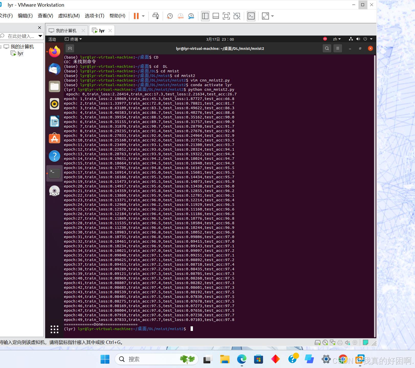
一、mnist_pytorch运行结果
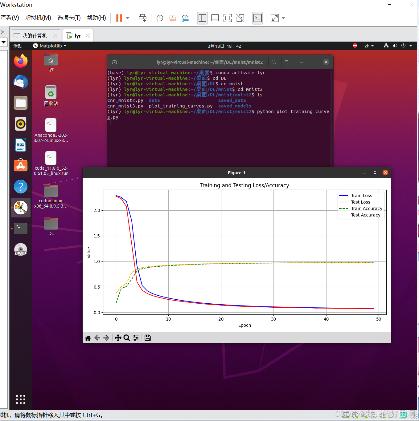
二、loss and acc 图+理论
说明:
train loss(训练损失):随着训练的进行,训练损失应该逐渐下降,表明模型在训练数据上的拟合能力增强。
test loss(测试损失):测试损失也应该逐渐下降,但如果模型过拟合,测试损失可能会在某个点开始上升。
train accuracy(训练准确率):训练准确率应该逐渐上升,表明模型在训练数据上的预测能力提高。
test accuracy(测试准确率):测试准确率也应该逐渐上升,但如果模型过拟合,测试准确率可能会停滞甚至下降。
1. 损失(Loss)
理论
a.定义:损失函数(Loss Function)用于衡量模型预测值与真实值之间的差异。在分类任务中,常用的损失函数是交叉熵损失(Cross-Entropy Loss)
b.作用:
损失值越小,说明模型的预测结果与真实值越接近。
训练过程中,优化器(如 SGD、Adam)的目标是最小化损失函数。
c.变化趋势:
在训练初期,损失值通常较高,随着训练的进行,损失值逐渐下降。
如果损失值在训练集上下降但在验证集上上升,可能是过拟合的迹象。
2. 准确率(Accuracy)
理论
a.定义:准确率是模型预测正确的样本数占总样本数的比例。
Number of Correct Predictions:模型预测正确的样本数。
Total Number of Predictions:总样本数。
b.作用:
准确率越高,说明模型的预测能力越强。
在分类任务中,准确率是最直观的评估指标。
c.变化趋势:
在训练初期,准确率通常较低,随着训练的进行,准确率逐渐上升。
如果训练集准确率持续上升但验证集准确率停滞或下降,可能是过拟合的迹象。
三、其他分类指标运算
机器学习
-
准确率(Accuracy)
-
定义与公式:预测正确的样本数占总样本数的比例,公式为Accuracy=TP+TN+FP+FNTP+TN。例如,在一个手写数字识别任务中,共有 1000 张数字图片,模型正确识别出了 900 张,那么准确率就是1000900=0.9。
-
适用场景与局限性:适用于样本分布较为均衡的情况,能直观地反映模型的整体分类性能。但当正负样本比例悬殊时,如正样本占比 99%,模型即使全部预测为正样本,准确率也会很高,却不能说明模型有效,此时准确率就具有一定的误导性。
-
-
精确率(Precision)
-
定义与公式:预测为正例的样本中,真正例的比例,公式为Precision=TP\TP+FP。例如,在一个疾病检测模型中,模型预测有 100 人患病,其中实际患病的有 80 人,那么精确率就是80\100=0.8。
-
适用场景与局限性:在一些对误判为正例代价较高的场景中非常重要,如金融诈骗检测,较高的精确率可以减少对正常交易的误判,降低不必要的调查成本。但如果召回率很低,即使精确率高,也可能遗漏很多真正的正例。
-
-
召回率(Recall)
-
定义与公式:实际为正例的样本中,被预测为正例的比例,公式为Recall=TP\TP+FN。例如,在一个癌症早期筛查模型中,实际有 100 名癌症患者,模型检测出了 60 名,召回率就是60\100=0.6。
-
适用场景与局限性:对于那些需要尽可能找出所有正例的场景至关重要,如疾病防控中的病例筛查,高召回率能确保大部分患者被及时发现。但如果只追求召回率,可能会导致大量误判,使精确率降低。
-
-
F1 值
-
定义与公式:精确率和召回率的调和平均数,公式为F1=2×(Precision×Recall)\(Precision+Recal)。例如,当精确率为 0.8,召回率为 0.6 时,F1=2×(0.8×0.6)\(0.8+0.6)≈0.69。
-
适用场景与局限性:综合了精确率和召回率,在样本不均衡、精确率和召回率此消彼长的情况下,能更全面地评估模型性能。但如果精确率和召回率都很低,F1 值也会较低,不能很好地反映模型在某些特定情况下的优势。
-
-
混淆矩阵
-
定义:是一个n×n的矩阵(n为类别数),用于展示分类模型的预测结果与真实标签之间的关系。矩阵的行表示真实类别,列表示预测类别。例如,在一个三分类问题中,混淆矩阵可能如下所示:
-
| 真实类别 \ 预测类别 | 类别 1 | 类别 2 | 类别 3 |
|---|---|---|---|
| 类别 1 | 80 | 10 | 10 |
| 类别 2 | 5 | 75 | 20 |
| 类别 3 | 3 | 12 | 85 |
-
适用场景与局限性:能清晰地展示出各类别的预测情况,包括正确分类和错误分类的样本数,帮助分析模型在不同类别上的性能表现,进而发现模型的优势和不足。但对于多类别问题,矩阵可能会比较复杂,难以直观地看出整体趋势。
深度学习
-
1.准确率、精确率、召回率、F1 值、ROC 曲线和 AUC
-
定义与计算方式:这些指标在深度学习中的定义与机器学习中基本相同。例如,在图像分类任务中,计算准确率时,同样是用正确分类的图像数量除以总图像数量。在计算 ROC 曲线时,通过不断调整分类阈值,得到不同阈值下的真正率(TPR)和假正率(FPR),从而绘制出曲线,AUC 则是曲线下的面积。
-
适用场景与特点:在深度学习的各种应用中广泛使用,如在医学图像分类中,通过 AUC 值可以评估模型对疾病类型判断的准确性;在自然语言处理的文本分类任务中,F1 值可以综合衡量模型对不同类别文本的分类效果。由于深度学习模型通常处理大规模、复杂的数据,这些指标能帮助评估模型在不同数据分布和特征情况下的性能。
-
-
对数损失(Log Loss)
-
定义与公式:也称为交叉熵损失,用于衡量模型预测的概率分布与真实标签的概率分布之间的差异。对于二分类问题,公式为
,其中y为真实标签(0 或 1),p为模型预测为正例的概率。对于多分类问题,公式为
,其中yi表示第i个类别对应的真实标签(0 或 1),pi表示模型预测第i个类别为正例的概率。
-
适用场景与特点:是深度学习中分类任务常用的损失函数,在训练模型时,通过最小化对数损失来调整模型的参数。它对预测概率与真实标签之间的差异非常敏感,能有效地引导模型学习到正确的概率分布,尤其适用于需要对类别进行概率估计的场景。
-
-
Hinge 损失
-
定义与公式:常用于支持向量机(SVM)等深度学习模型中,特别是在二分类问题中。公式为
,其中y为真实标签(+1或−1),f(x)为模型的预测得分。
-
适用场景与特点:它的目标是使正确分类的样本距离决策边界尽可能远,而错误分类的样本受到惩罚。Hinge 损失对于离群点相对不敏感,能有效防止模型过拟合,在一些对模型泛化能力要求较高的场景中表现较好,如在处理具有复杂边界的分类问题时,能使模型学习到更鲁棒的决策边界。
-
在原有的基础上添加更多的分类指标,如精确率(Precision)、召回率(Recall)和 F1 值。代码如下
import os
import torch
import torchvision
import torch.nn as nn
from torchvision import datasets, transforms
import torch.nn.functional as F
from sklearn.metrics import precision_score, recall_score, f1_score
import numpy as np


# 数据预处理
transformation = transforms.Compose([
    transforms.ToTensor(),
    transforms.Normalize((0.5,), (0.5,))  # MNIST是单通道图像,均值和标准差为(0.5,)
])

# 加载MNIST数据集
train_dataset = torchvision.datasets.MNIST('data',
                                           train=True,
                                           transform=transformation,
                                           download=True)

test_dataset = torchvision.datasets.MNIST('data',
                                          train=False,
                                          transform=transformation,
                                          download=True)

# 创建数据加载器
train_dl = torch.utils.data.DataLoader(train_dataset, batch_size=64, shuffle=True)
test_dl = torch.utils.data.DataLoader(test_dataset, batch_size=64, shuffle=True)

# 构建CNN模型
class Model(nn.Module):
    def __init__(self):
        super(Model, self).__init__()
        self.conv1 = nn.Conv2d(1, 6, 5)  # 输入通道1,输出通道6,卷积核大小5x5
        self.conv2 = nn.Conv2d(6, 16, 3)  # 输入通道6,输出通道16,卷积核大小3x3
        self.pool = nn.MaxPool2d((2, 2))  # 最大池化层,2x2
        self.linear_1 = nn.Linear(16 * 5 * 5, 256)  # 全连接层,输入16*5*5,输出256
        self.linear_2 = nn.Linear(256, 10)  # 全连接层,输入256,输出10(10个类别)

    def forward(self, input):
        x = F.relu(self.conv1(input))  # 卷积层1 + ReLU激活
        x = self.pool(x)  # 池化层
        x = F.relu(self.conv2(x))  # 卷积层2 + ReLU激活
        x = self.pool(x)  # 池化层
        x = x.view(x.size(0), -1)  # 展平操作,将多维张量展平为一维
        x = F.relu(self.linear_1(x))  # 全连接层1 + ReLU激活
        x = self.linear_2(x)  # 全连接层2
        return x


# 选择设备
device = 'cuda' if torch.cuda.is_available() else 'cpu'
model = Model().to(device)
loss_fn = torch.nn.CrossEntropyLoss()  # 交叉熵损失函数
opt = torch.optim.SGD(model.parameters(), lr=0.001)  # 随机梯度下降优化器


# 训练函数
def train(dl, model, loss_fn, optimizer):
    size = len(dl.dataset)  # 数据集的大小
    num_batches = len(dl)

    train_loss, correct = 0, 0
    all_preds = []
    all_labels = []

    for x, y in dl:
        x, y = x.to(device), y.to(device)
        pred = model(x)
        loss = loss_fn(pred, y)
        optimizer.zero_grad()  # 梯度清零
        loss.backward()
        optimizer.step()
        with torch.no_grad():
            correct += (pred.argmax(1) == y).type(torch.float).sum().item()
            train_loss += loss.item()
            all_preds.extend(pred.argmax(1).cpu().numpy())
            all_labels.extend(y.cpu().numpy())

    correct /= size
    train_loss /= num_batches

    precision = precision_score(all_labels, all_preds, average='macro')
    recall = recall_score(all_labels, all_preds, average='macro')
    f1 = f1_score(all_labels, all_preds, average='macro')

    return correct, train_loss, precision, recall, f1


# 测试函数
def test(test_dl, model, loss_fn):
    size = len(test_dl.dataset)  # 数据集的大小
    num_batches = len(test_dl)

    test_loss, correct = 0, 0
    all_preds = []
    all_labels = []

    with torch.no_grad():
        for x, y in test_dl:
            x, y = x.to(device), y.to(device)
            pred = model(x)
            loss = loss_fn(pred, y)
            test_loss += loss.item()
            correct += (pred.argmax(1) == y).type(torch.float).sum().item()
            all_preds.extend(pred.argmax(1).cpu().numpy())
            all_labels.extend(y.cpu().numpy())

    correct /= size
    test_loss /= num_batches

    precision = precision_score(all_labels, all_preds, average='macro')
    recall = recall_score(all_labels, all_preds, average='macro')
    f1 = f1_score(all_labels, all_preds, average='macro')

    return correct, test_loss, precision, recall, f1


# 创建保存模型的目录
if not os.path.exists('saved_models'):
    os.makedirs('saved_models')

# 创建保存训练数据的目录
if not os.path.exists('saved_data'):
    os.makedirs('saved_data')


# 训练和测试循环
def fit(epochs, train_dl, test_dl, model, loss_fn, opt):
    train_losses = []
    train_accs = []
    train_precisions = []
    train_recalls = []
    train_f1s = []

    test_losses = []
    test_accs = []
    test_precisions = []
    test_recalls = []
    test_f1s = []

    for epoch in range(epochs):
        epoch_acc, epoch_loss, epoch_train_precision, epoch_train_recall, epoch_train_f1 = train(
            train_dl, model, loss_fn, opt)
        epoch_test_acc, epoch_test_loss, epoch_test_precision, epoch_test_recall, epoch_test_f1 = test(
            test_dl, model, loss_fn)

        train_losses.append(epoch_loss)
        train_accs.append(epoch_acc)
        train_precisions.append(epoch_train_precision)
        train_recalls.append(epoch_train_recall)
        train_f1s.append(epoch_train_f1)

        test_losses.append(epoch_test_loss)
        test_accs.append(epoch_test_acc)
        test_precisions.append(epoch_test_precision)
        test_recalls.append(epoch_test_recall)
        test_f1s.append(epoch_test_f1)

        template = ("epoch:{:2d}, train_loss:{:.5f}, train_acc:{:.1f}%, train_precision:{:.1f}%, train_recall:{:.1f}%, train_f1:{:.1f}%, "
                    "test_loss:{:.5f}, test_acc:{:.1f}%, test_precision:{:.1f}%, test_recall:{:.1f}%, test_f1:{:.1f}%")
        print(template.format(epoch, epoch_loss, epoch_acc * 100, epoch_train_precision * 100,
                              epoch_train_recall * 100, epoch_train_f1 * 100,
                              epoch_test_loss, epoch_test_acc * 100, epoch_test_precision * 100,
                              epoch_test_recall * 100, epoch_test_f1 * 100))

    # 保存模型
    model_path = 'saved_models/mnist_cnn_model.pth'
    torch.save(model.state_dict(), model_path)
    print(f"Model saved to {model_path}")

    # 保存训练数据
    train_data = {
        'train_loss': train_losses,
        'train_acc': train_accs,
        'train_precision': train_precisions,
        'train_recall': train_recalls,
        'train_f1': train_f1s,
        'test_loss': test_losses,
        'test_acc': test_accs,
        'test_precision': test_precisions,
        'test_recall': test_recalls,
        'test_f1': test_f1s
    }
    data_path = 'saved_data/training_data.pth'
    torch.save(train_data, data_path)
    print(f"Training data saved to {data_path}")

    print("=============Done===============")
    return train_losses, train_accs, train_precisions, train_recalls, train_f1s, \
        test_losses, test_accs, test_precisions, test_recalls, test_f1s


# 开始训练
train_losses, train_accs, train_precisions, train_recalls, train_f1s, \
    test_losses, test_accs, test_precisions, test_recalls, test_f1s = fit(50, train_dl, test_dl, model, loss_fn, opt)
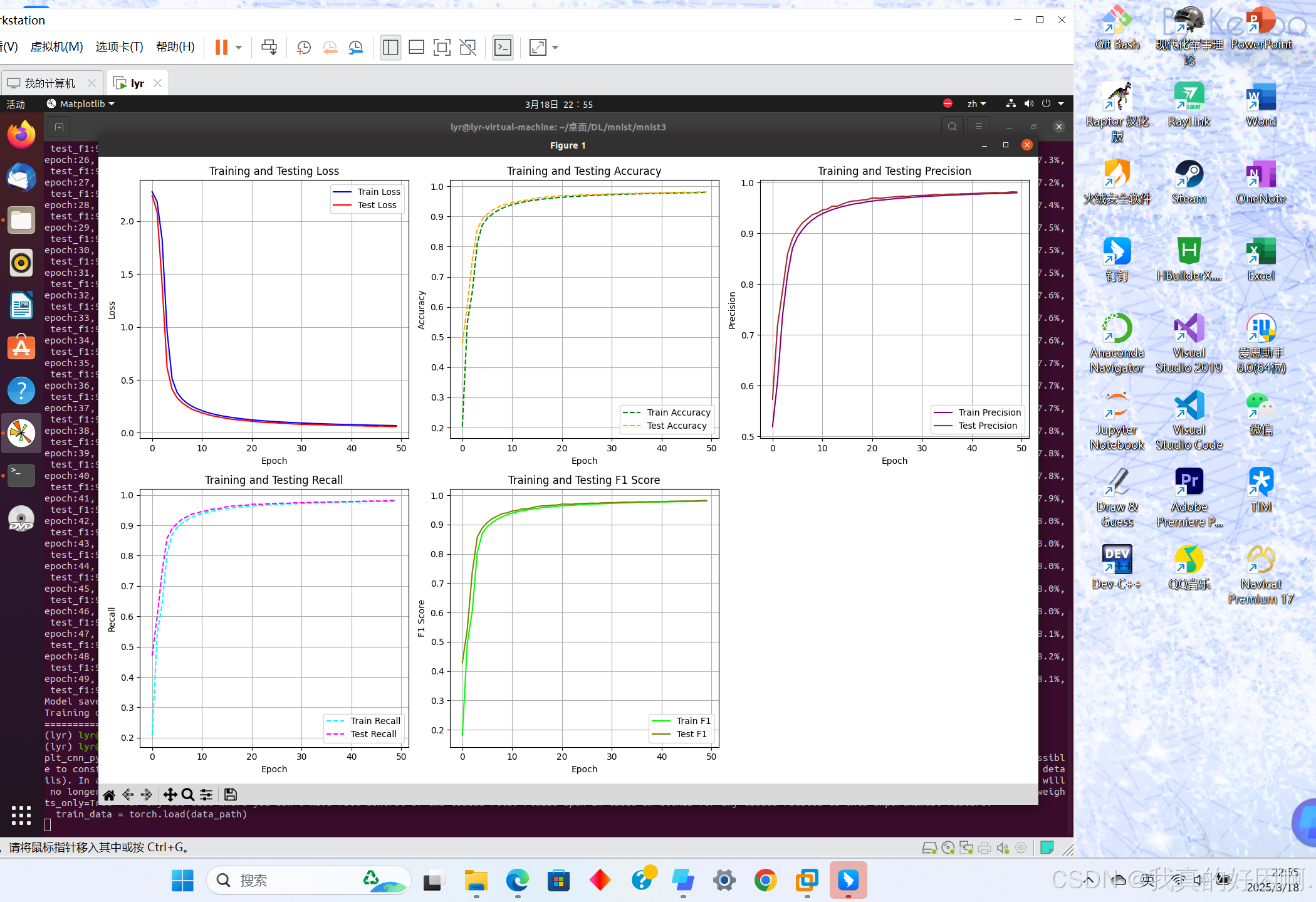
运行结果和图形绘制
绘制结果代码
import os
import torch
import matplotlib.pyplot as plt  # 用于绘图

# 从文件中加载训练数据
data_path ='saved_data/training_data.pth'  # 训练数据文件路径
# 添加安全全局变量,这里假设你的数据中没有自定义的特殊对象,如果有需要根据实际情况添加
torch.serialization.add_safe_globals({})
train_data = torch.load(data_path)

# 提取训练和测试的损失、准确率、精确率、召回率和 F1 值
train_loss = train_data['train_loss']
train_acc = train_data['train_acc']
train_precision = train_data['train_precision']
train_recall = train_data['train_recall']
train_f1 = train_data['train_f1']

test_loss = train_data['test_loss']
test_acc = train_data['test_acc']
test_precision = train_data['test_precision']
test_recall = train_data['test_recall']
test_f1 = train_data['test_f1']

# 获取训练的 epoch 数量
epochs = len(train_loss)

# 绘制损失、准确率、精确率、召回率和 F1 值曲线
plt.figure(figsize=(15, 10))  # 设置图表大小

# 绘制损失曲线
plt.subplot(2, 3, 1)
plt.plot(range(epochs), train_loss, label='Train Loss', color='blue', linestyle='-')
plt.plot(range(epochs), test_loss, label='Test Loss', color='red', linestyle='-')
plt.xlabel('Epoch')
plt.ylabel('Loss')
plt.title('Training and Testing Loss')
plt.legend(loc='upper right')
plt.grid(True)

# 绘制准确率曲线
plt.subplot(2, 3, 2)
plt.plot(range(epochs), train_acc, label='Train Accuracy', color='green', linestyle='--')
plt.plot(range(epochs), test_acc, label='Test Accuracy', color='orange', linestyle='--')
plt.xlabel('Epoch')
plt.ylabel('Accuracy')
plt.title('Training and Testing Accuracy')
plt.legend(loc='lower right')
plt.grid(True)

# 绘制精确率曲线
plt.subplot(2, 3, 3)
plt.plot(range(epochs), train_precision, label='Train Precision', color='purple', linestyle='-')
plt.plot(range(epochs), test_precision, label='Test Precision', color='brown', linestyle='-')
plt.xlabel('Epoch')
plt.ylabel('Precision')
plt.title('Training and Testing Precision')
plt.legend(loc='lower right')
plt.grid(True)

# 绘制召回率曲线
plt.subplot(2, 3, 4)
plt.plot(range(epochs), train_recall, label='Train Recall', color='cyan', linestyle='--')
plt.plot(range(epochs), test_recall, label='Test Recall', color='magenta', linestyle='--')
plt.xlabel('Epoch')
plt.ylabel('Recall')
plt.title('Training and Testing Recall')
plt.legend(loc='lower right')
plt.grid(True)

# 绘制 F1 值曲线
plt.subplot(2, 3, 5)
plt.plot(range(epochs), train_f1, label='Train F1', color='lime', linestyle='-')
plt.plot(range(epochs), test_f1, label='Test F1', color='olive', linestyle='-')
plt.xlabel('Epoch')
plt.ylabel('F1 Score')
plt.title('Training and Testing F1 Score')
plt.legend(loc='lower right')
plt.grid(True)

plt.tight_layout()  # 调整布局
plt.show()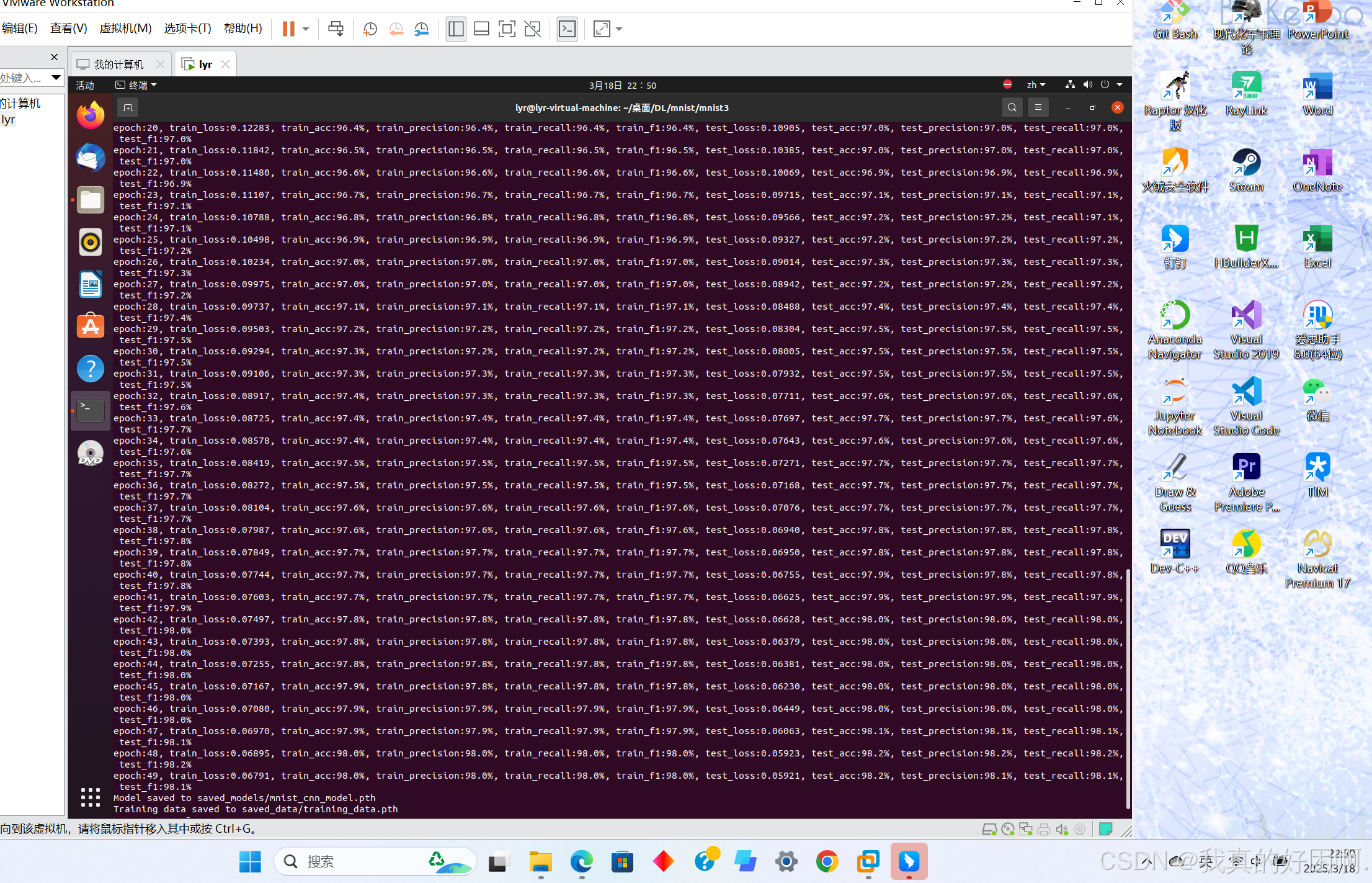
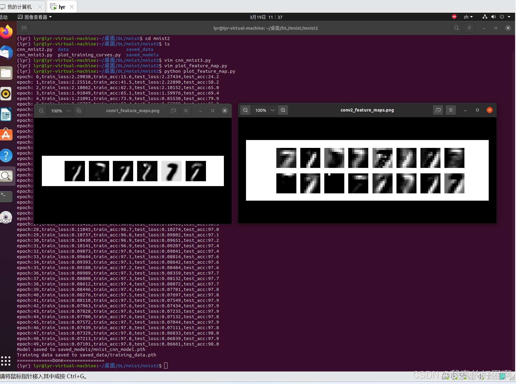
四、feature map图
feature map(特征图):在cnn的每个卷积层,数据都是以三维形式存在的。你可以把它看成许多个二维图片叠在一起(像豆腐皮一样),其中每一个称为一个feature map。
输入层:在输入层,如果是灰度图片,那就只有一个feature map;
如果是彩色图片,一般就是3个feature map(红绿蓝)。
其它层:层与层之间会有若干个卷积核(kernel)(也称为过滤器),上一层每个feature map跟每个卷积核做卷积,都会产生下一层的一个feature map,有N个卷积核,下层就会产生N个feather map。
如何计算?
主要由卷积和池化层
- 卷积层计算
- 卷积核滑动:在卷积层中,通过将卷积核在输入数据上进行滑动,对每个位置进行卷积操作。卷积核的大小通常为奇数,如\(3\times3\)、\(5\times5\)等,它代表了在输入数据的局部区域上进行特征提取的窗口。
- 计算方式:对于输入的二维图像数据(假设通道数为C),卷积核的通道数也为C,且具有一定的深度K(即卷积核的个数)。在滑动过程中,卷积核与输入数据对应位置的元素相乘并求和,得到输出特征图上的一个像素值。具体来说,对于输入特征图X,卷积核W,输出特征图Y,在位置(i,j)处的计算为
,其中m和n是卷积核内元素的坐标,c是通道索引。
- 偏置与激活:在完成上述计算后,通常会为每个卷积核添加一个偏置项b,然后将结果通过一个激活函数,如 ReLU(Rectified Linear Unit)函数\(f(x)=\max(0, x)\),得到最终的特征图。即。
- 池化层计算
- 作用与方式:池化层主要用于对卷积层得到的特征图进行下采样,以减少数据量和计算量,同时保留主要的特征信息。常见的池化方式有最大池化(Max Pooling)和平均池化(Average Pooling)。
- 最大池化计算:最大池化是在一个固定大小的池化窗口内取最大值作为输出。例如,池化窗口大小为\(2\times2\),步长为2,则将特征图划分为若干个\(2\times2\)的小块,每个小块中取最大值作为该区域池化后的结果,从而得到下采样后的特征图。
- 平均池化计算:平均池化则是在池化窗口内计算平均值作为输出。同样以\(2\times2\)的池化窗口为例,将每个小块内的元素值求平均,得到池化后的特征图。
示例代码
import os
import torch
import torchvision
import torch.nn as nn
from torchvision import datasets, transforms
import torch.nn.functional as F
import matplotlib.pyplot as plt


# 数据预处理
transformation = transforms.Compose([
    transforms.ToTensor(),
    transforms.Normalize((0.5,), (0.5,))  # MNIST是单通道图像,均值和标准差为(0.5,)
])

# 加载MNIST数据集
train_dataset = torchvision.datasets.MNIST('data',
                                           train=True,
                                           transform=transformation,
                                           download=True)

test_dataset = torchvision.datasets.MNIST('data',
                                          train=False,
                                          transform=transformation,
                                          download=True)

# 创建数据加载器
train_dl = torch.utils.data.DataLoader(train_dataset, batch_size=64, shuffle=True)
test_dl = torch.utils.data.DataLoader(test_dataset, batch_size=64, shuffle=True)

# 构建CNN模型
class Model(nn.Module):
    def __init__(self):
        super(Model, self).__init__()
        self.conv1 = nn.Conv2d(1, 6, 5)  # 输入通道1,输出通道6,卷积核大小5x5
        self.conv2 = nn.Conv2d(6, 16, 3)  # 输入通道6,输出通道16,卷积核大小3x3
        self.pool = nn.MaxPool2d((2, 2))  # 最大池化层,2x2
        self.linear_1 = nn.Linear(16 * 5 * 5, 256)  # 全连接层,输入16*5*5,输出256
        self.linear_2 = nn.Linear(256, 10)  # 全连接层,输入256,输出10(10个类别)

    def forward(self, input):
        x = F.relu(self.conv1(input))  # 卷积层1 + ReLU激活
        conv1_output = x
        x = self.pool(x)  # 池化层
        x = F.relu(self.conv2(x))  # 卷积层2 + ReLU激活
        conv2_output = x
        x = self.pool(x)  # 池化层
        x = x.view(x.size(0), -1)  # 展平操作,将多维张量展平为一维
        x = F.relu(self.linear_1(x))  # 全连接层1 + ReLU激活
        x = self.linear_2(x)  # 全连接层2
        return x, conv1_output, conv2_output


# 选择设备
device = 'cuda' if torch.cuda.is_available() else 'cpu'
model = Model().to(device)
loss_fn = torch.nn.CrossEntropyLoss()  # 交叉熵损失函数
opt = torch.optim.SGD(model.parameters(), lr=0.001)  # 随机梯度下降优化器

# 训练函数
def train(dl, model, loss_fn, optimizer):
    size = len(dl.dataset)  # 数据集的大小
    num_batches = len(dl)

    train_loss, correct = 0, 0

    for x, y in dl:
        x, y = x.to(device), y.to(device)
        pred, _, _ = model(x)
        loss = loss_fn(pred, y)
        optimizer.zero_grad()  # 梯度清零
        loss.backward()
        optimizer.step()
        with torch.no_grad():
            correct += (pred.argmax(1) == y).type(torch.float).sum().item()
            train_loss += loss.item()
    correct /= size
    train_loss /= num_batches
    return correct, train_loss


# 测试函数
def test(test_dl, model, loss_fn):
    size = len(test_dl.dataset)  # 数据集的大小
    num_batches = len(test_dl)

    test_loss, correct = 0, 0

    with torch.no_grad():
        for x, y in test_dl:
            x, y = x.to(device), y.to(device)
            pred, _, _ = model(x)
            loss = loss_fn(pred, y)
            test_loss += loss.item()
            correct += (pred.argmax(1) == y).type(torch.float).sum().item()
        correct /= size
        test_loss /= num_batches
        return correct, test_loss


# 创建保存模型的目录
if not os.path.exists('saved_models'):
    os.makedirs('saved_models')

# 创建保存训练数据的目录
if not os.path.exists('saved_data'):
    os.makedirs('saved_data')

# 训练和测试循环
def fit(epochs, train_dl, test_dl, model, loss_fn, opt):
    train_loss = []
    train_acc = []
    test_loss = []
    test_acc = []
    for epoch in range(epochs):
        epoch_acc, epoch_loss = train(train_dl, model, loss_fn, opt)
        epoch_test_acc, epoch_test_loss = test(test_dl, model, loss_fn)

        train_loss.append(epoch_loss)
        train_acc.append(epoch_acc)

        test_loss.append(epoch_test_loss)
        test_acc.append(epoch_test_acc)

        template = ("epoch:{:2d},train_loss:{:.5f},train_acc:{:.1f},test_loss:{:.5f},test_acc:{:.1f}")
        print(template.format(epoch, epoch_loss, epoch_acc * 100, epoch_test_loss, epoch_test_acc * 100))

    # 保存模型
    model_path = 'saved_models/mnist_cnn_model.pth'
    torch.save(model.state_dict(), model_path)
    print(f"Model saved to {model_path}")

    # 保存训练数据
    train_data = {
        'train_loss': train_loss,
        'train_acc': train_acc,
        'test_loss': test_loss,
        'test_acc': test_acc
    }
    data_path = 'saved_data/training_data.pth'
    torch.save(train_data, data_path)
    print(f"Training data saved to {data_path}")

    print("=============Done===============")
    return train_loss, train_acc, test_loss, test_acc


# 生成特征图
def generate_feature_maps(model, test_dl, device):
    with torch.no_grad():
        for x, y in test_dl:
            x, y = x.to(device), y.to(device)
            _, conv1_output, conv2_output = model(x)

            # 选择第一个样本的特征图
            conv1_output = conv1_output[0].cpu().numpy()
            conv2_output = conv2_output[0].cpu().numpy()

            # 绘制第一个卷积层的特征图
            num_filters_conv1 = conv1_output.shape[0]
            fig, axes = plt.subplots(1, num_filters_conv1, figsize=(num_filters_conv1, 1))
            for i in range(num_filters_conv1):
                axes[i].imshow(conv1_output[i], cmap='gray')
                axes[i].axis('off')
            plt.savefig('saved_data/conv1_feature_maps.png')
            plt.close()

            # 绘制第二个卷积层的特征图
            num_filters_conv2 = conv2_output.shape[0]
            fig, axes = plt.subplots(2, num_filters_conv2 // 2, figsize=(num_filters_conv2 // 2, 2))
            axes = axes.flatten()
            for i in range(num_filters_conv2):
                axes[i].imshow(conv2_output[i], cmap='gray')
                axes[i].axis('off')
            plt.savefig('saved_data/conv2_feature_maps.png')
            plt.close()
            break


# 开始训练
train_loss, train_acc, test_loss, test_acc = fit(50, train_dl, test_dl, model, loss_fn, opt)

# 生成特征图
generate_feature_maps(model, test_dl, device)
结果:


 1070
1070

 被折叠的 条评论
为什么被折叠?
被折叠的 条评论
为什么被折叠?
 到【灌水乐园】发言


