


CNN(练习数据集)
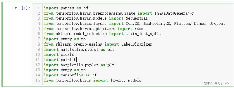
- 1.导包:
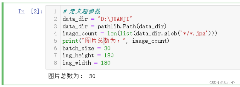
- 2.导入数据集:
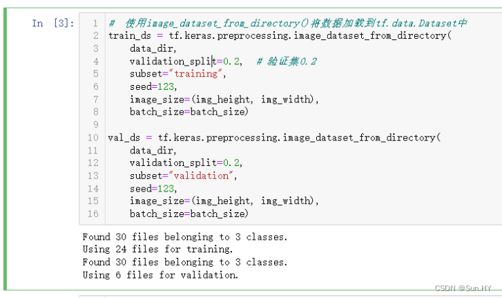
- 3. 使用image_dataset_from_directory()将数据加载tf.data.Dataset中:
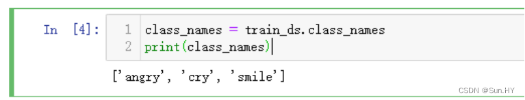
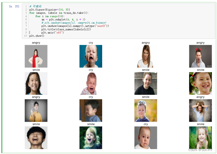
- 4. 查看数据集中的一部分图像,以及它们对应的标签:
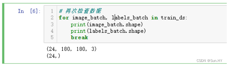
- 5.迭代数据集 train_ds,以便查看第一批图像和标签的形状:
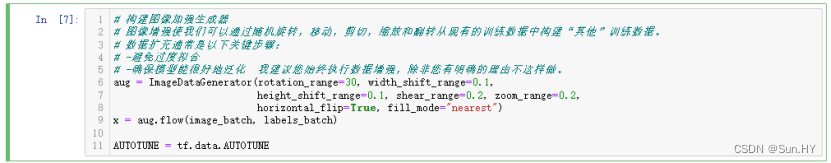
- 6.使用TensorFlow的ImageDataGenerator类来创建一个数据增强的对象:
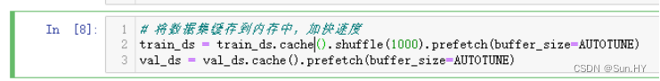
- 7.将数据集缓存到内存中,加快速度:
- 8. 通过卷积层和池化层提取特征,再通过全连接层进行分类:
- 9.打印网络结构:
- 10.设置优化器,定义了训练轮次和批量大小:
- 11.训练数据集:
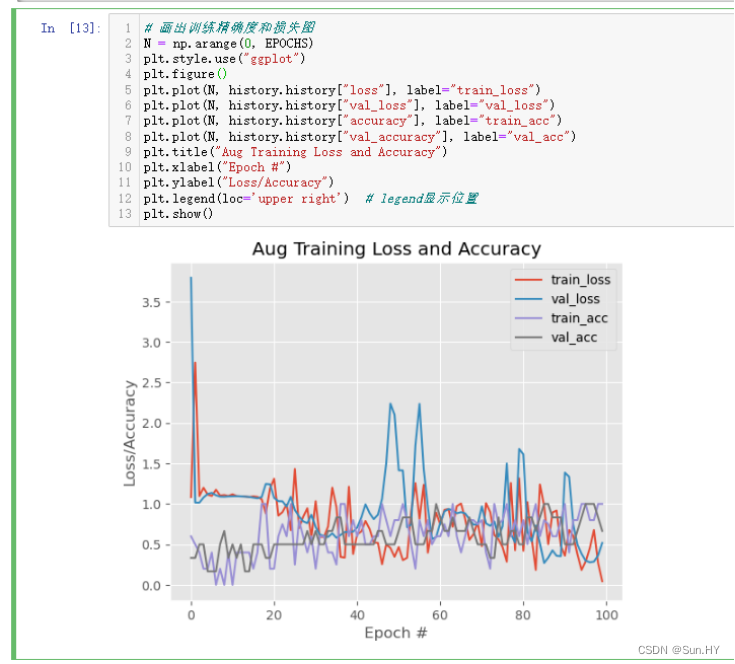
- 12.画出图像:
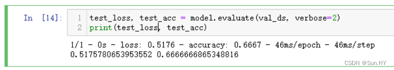
- 13.评估您的模型在验证数据集的性能:
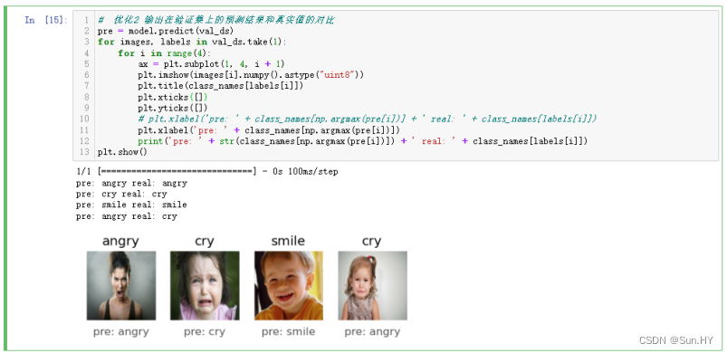
- 14.输出在验证集上的预测结果和真实值的对比:
- 15.输出可视化报表:
- 在网上寻找一个新的数据集,自己进行训练
1.导包:
import pandas as pd
from tensorflow.keras.preprocessing.image import ImageDataGenerator
from tensorflow.keras.models import Sequential
from tensorflow.keras.layers import Conv2D, MaxPooling2D, Flatten, Dense, Dropout
from tensorflow.keras.optimizers import Adam
from sklearn.model_selection import train_test_split
import numpy as np
from sklearn.preprocessing import LabelBinarizer
import matplotlib.pyplot as plt
import pickle
import pathlib
import matplotlib.pyplot as plt
import numpy as np
import tensorflow as tf
from tensorflow.keras import layers, models
输出结果:
2.导入数据集:
# 定义超参数
data_dir = "D:\JUANJI"
data_dir = pathlib.Path(data_dir)
image_count = len(list(data_dir.glob('*/*.jpg')))
print("图片总数为:", image_count)
batch_size = 30
img_height = 180
img_width = 180
输出结果:
3. 使用image_dataset_from_directory()将数据加载tf.data.Dataset中:
#  使用image_dataset_from_directory()将数据加载到tf.data.Dataset中
train_ds = tf.keras.preprocessing.image_dataset_from_directory(
    data_dir,
    validation_split=0.2,  # 验证集0.2
    subset="training",
    seed=123,
    image_size=(img_height, img_width),
    batch_size=batch_size)

val_ds = tf.keras.preprocessing.image_dataset_from_directory(
    data_dir,
    validation_split=0.2,
    subset="validation",
    seed=123,
    image_size=(img_height, img_width),
    batch_size=batch_size)
输出结果:
4. 查看数据集中的一部分图像,以及它们对应的标签:
class_names = train_ds.class_names
print(class_names)
# 可视化
plt.figure(figsize=(16, 8))
for images, labels in train_ds.take(1):
    for i in range(16):
        ax = plt.subplot(4, 4, i + 1)
        # plt.imshow(images[i], cmap=plt.cm.binary)
        plt.imshow(images[i].numpy().astype("uint8"))
        plt.title(class_names[labels[i]])
        plt.axis("off")
plt.show()
输出结果:
5.迭代数据集 train_ds,以便查看第一批图像和标签的形状:
for image_batch, labels_batch in train_ds:
    print(image_batch.shape)
    print(labels_batch.shape)
    break
输出结果:
6.使用TensorFlow的ImageDataGenerator类来创建一个数据增强的对象:
aug = ImageDataGenerator(rotation_range=30, width_shift_range=0.1,
            height_shift_range=0.1, shear_range=0.2, zoom_range=0.2,
            horizontal_flip=True, fill_mode="nearest")
x = aug.flow(image_batch, labels_batch)
AUTOTUNE = tf.data.AUTOTUNE
输出结果:
7.将数据集缓存到内存中,加快速度:
train_ds = train_ds.cache().shuffle(1000).prefetch(buffer_size=AUTOTUNE)
val_ds = val_ds.cache().prefetch(buffer_size=AUTOTUNE)
输出结果:
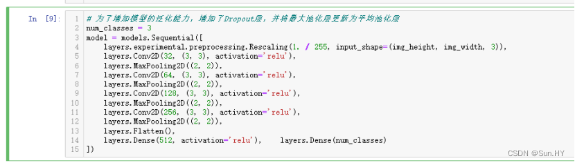
8. 通过卷积层和池化层提取特征,再通过全连接层进行分类:
# 为了增加模型的泛化能力,增加了Dropout层,并将最大池化层更新为平均池化层
num_classes = 3
model = models.Sequential([
    layers.experimental.preprocessing.Rescaling(1./255,input_shape=(img_height,img_width, 3)),
    layers.Conv2D(32, (3, 3), activation='relu'),
    layers.MaxPooling2D((2, 2)),
    layers.Conv2D(64, (3, 3), activation='relu'),
    layers.MaxPooling2D((2, 2)),
    layers.Conv2D(128, (3, 3), activation='relu'),
    layers.MaxPooling2D((2, 2)),
    layers.Conv2D(256, (3, 3), activation='relu'),
    layers.MaxPooling2D((2, 2)),
    layers.Flatten(),
    layers.Dense(512, activation='relu'),
    layers.Dense(num_classes)
])
输出结果:
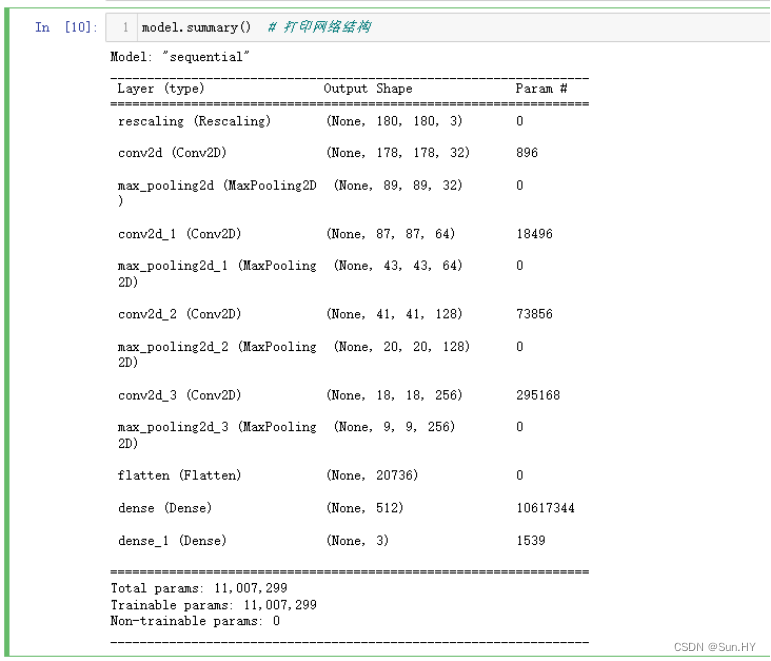
9.打印网络结构:
model.summary()
输出结果:
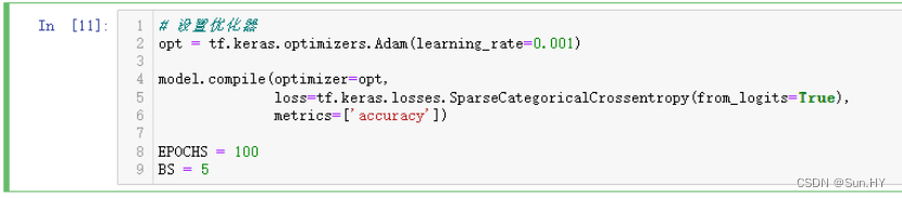
10.设置优化器,定义了训练轮次和批量大小:
# 设置优化器
opt = tf.keras.optimizers.Adam(learning_rate=0.001)

model.compile(optimizer=opt,
              loss=tf.keras.losses.SparseCategoricalCrossentropy(from_logits=True),
              metrics=['accuracy'])

EPOCHS = 100
BS = 5
输出结果:
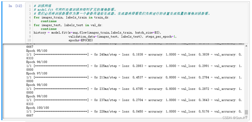
11.训练数据集:
# 训练网络
# model.fit 可同时处理训练和即时扩充的增强数据。
# 我们必须将训练数据作为第一个参数传递给生成器。生成器将根据我们先前进行的设置生成批量的增强训练数据。
for images_train, labels_train in train_ds:
    continue
for images_test, labels_test in val_ds:
    continue
history = model.fit(x=aug.flow(images_train,labels_train, batch_size=BS),
                 validation_data=(images_test,labels_test),
steps_per_epoch=1,epochs=EPOCHS)
输出结果:
12.画出图像:
# 画出训练精确度和损失图
N = np.arange(0, EPOCHS)
plt.style.use("ggplot")
plt.figure()
plt.plot(N, history.history["loss"], label="train_loss")
plt.plot(N, history.history["val_loss"], label="val_loss")
plt.plot(N, history.history["accuracy"], label="train_acc")
plt.plot(N, history.history["val_accuracy"], label="val_acc")
plt.title("Aug Training Loss and Accuracy")
plt.xlabel("Epoch #")
plt.ylabel("Loss/Accuracy")
plt.legend(loc='upper right')  # legend显示位置
plt.show()
输出结果:
13.评估您的模型在验证数据集的性能:
test_loss, test_acc = model.evaluate(val_ds, verbose=2)
print(test_loss, test_acc)
输出结果:
14.输出在验证集上的预测结果和真实值的对比:
#  优化2 输出在验证集上的预测结果和真实值的对比
pre = model.predict(val_ds)
for images, labels in val_ds.take(1):
    for i in range(4):
        ax = plt.subplot(1, 4, i + 1)
        plt.imshow(images[i].numpy().astype("uint8"))
        plt.title(class_names[labels[i]])
        plt.xticks([])
        plt.yticks([])
        # plt.xlabel('pre: ' + class_names[np.argmax(pre[i])] + ' real: ' + class_names[labels[i]])
        plt.xlabel('pre: ' + class_names[np.argmax(pre[i])])
        print('pre: ' + str(class_names[np.argmax(pre[i])]) + ' real: ' + class_names[labels[i]])
plt.show()
输出结果:
15.输出可视化报表:
print(labels_test)
print(labels)
print(pre)
print(class_names)
from sklearn.metrics import classification_report
# 优化1 输出可视化报表
print(classification_report(labels_test,
                          pre.argmax(axis=1),
target_names=class_names))
输出结果:


 1万+
1万+


 被折叠的 条评论
为什么被折叠?
被折叠的 条评论
为什么被折叠?
 到【灌水乐园】发言


