


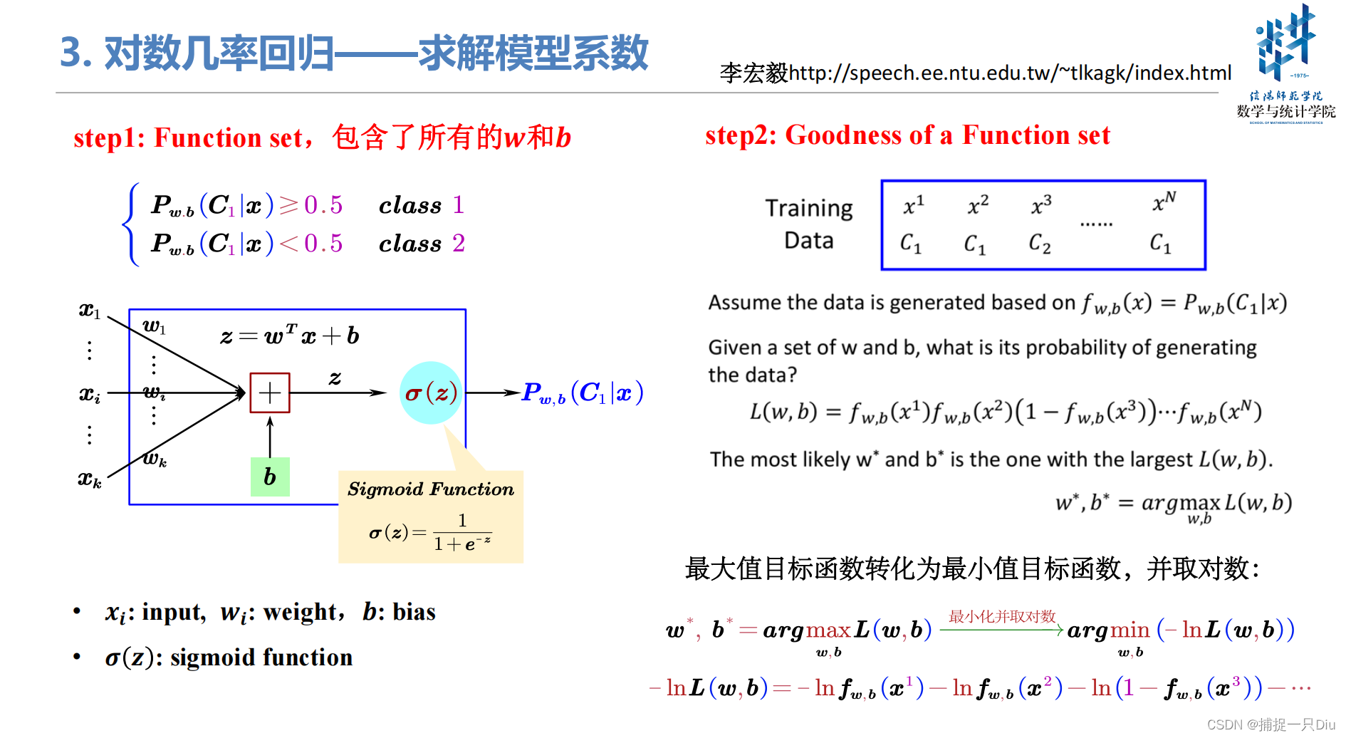
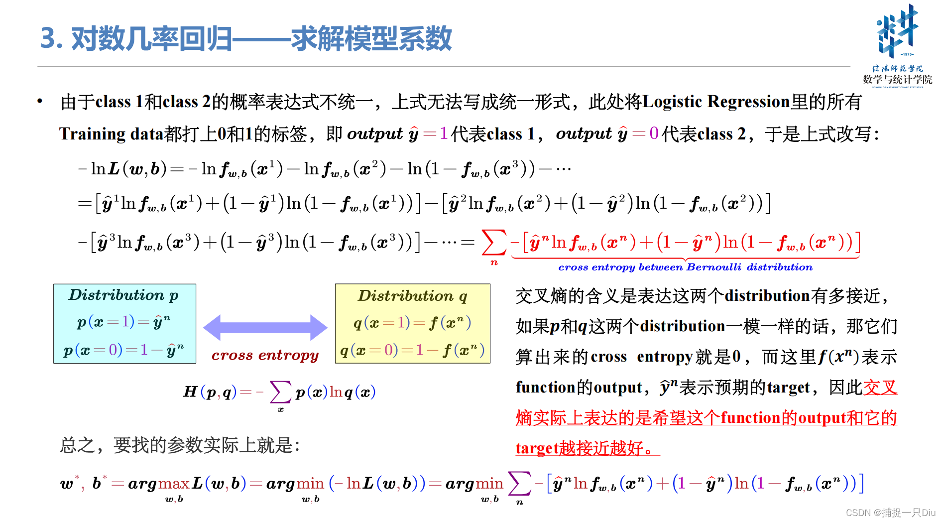
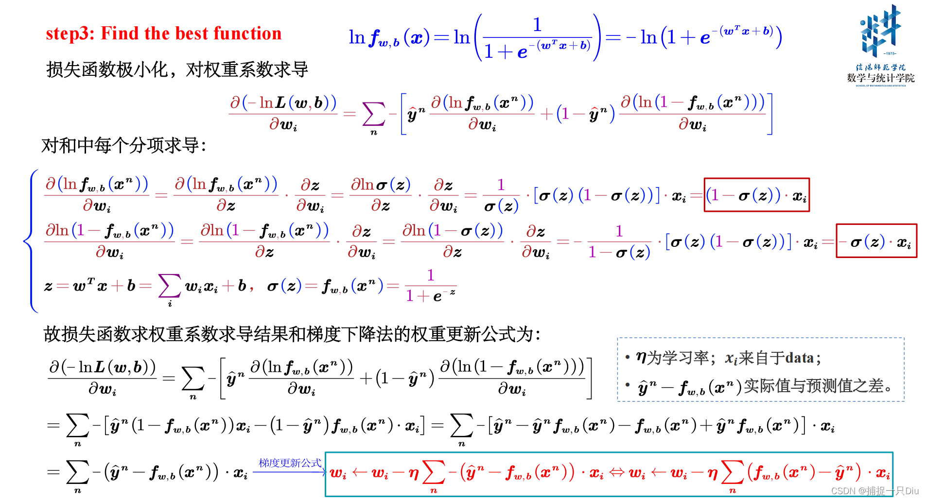
Logistic回归(二分类)
logistic_regression_class2.py
import numpy as np
import matplotlib.pyplot as plt


class LogisticRegression:
    """
    逻辑回归,采用梯度下降算法 + 正则化,交叉熵损失函数,实现二分类
    """
    def __init__(self, fit_intercept=True, normalize=True, alpha=0.05, eps=1e-10,
                 max_epochs=300, batch_size=20, l1_ratio=None, l2_ratio=None, en_rou=None):
        """
        :param eps: 提前停止训练的精度要求,按照两次训练损失的绝对值差小于eps,停止训练
        :param fit_intercept: 是否训练偏置项
        :param normalize: 是否标准化
        :param alpha: 学习率
        :param max_epochs: 最大迭代次数
        :param batch_size: 批量大小,若为1,则为随机梯度,若为训练集样本量,则为批量梯度,否则为小批量梯度
        :param l1_ratio: LASSO回归惩罚项系数
        :param l2_ratio: 岭回归惩罚项系数
        :param en_rou: 弹性网络权衡L1和L2的系数
        """
        self.fit_intercept = fit_intercept  # 线性模型的常数项。也即偏置bias,模型中的theta0
        self.normalize = normalize  # 是否标准化数据
        self.alpha = alpha  # 学习率
        self.eps = eps  # 提前停止训练
        if l1_ratio:
            if l1_ratio < 0:
                raise ValueError("惩罚项系数不能为负数")
        self.l1_ratio = l1_ratio  # LASSO回归惩罚项系数
        if l2_ratio:
            if l2_ratio < 0:
                raise ValueError("惩罚项系数不能为负数")
        self.l2_ratio = l2_ratio  # 岭回归惩罚项系数
        if en_rou:
            if en_rou > 1 or en_rou < 0:
                raise ValueError("弹性网络权衡系数范围在[0, 1]")
        self.en_rou = en_rou  # 弹性网络权衡L1和L2的系数
        self.max_epochs = max_epochs
        self.batch_size = batch_size
        self.theta = None  # 训练权重系数
        if normalize:
            self.feature_mean, self.feature_std = None, None  # 特征的均值,标准方差
        self.n_samples, self.n_features = 0, 0  # 样本量和特征数
        self.train_loss, self.test_loss = [], []  # 存储训练过程中的训练损失和测试损失

    def init_theta_params(self, n_features):
        """
        初始化参数
        如果训练偏置项,也包含了bias的初始化
        :return:
        """
        self.theta = np.random.randn(n_features, 1) * 0.1

    @staticmethod
    def sigmoid(x):
        """
        sigmoid函数,为避免上溢或下溢,对参数x做限制
        :param x: 可能是标量数据,也可能是数组
        :return:
        """
        x = np.asarray(x)  # 为避免标量值的布尔索引出错,转换为数组
        x[x > 30.0] = 30.0  # 避免下溢
        x[x < -50] = -50.0  # 避免上溢
        return 1 / (1 + np.exp(-x))

    @staticmethod
    def sign_func(weight):
        """
        符号函数,针对L1正则化
        :param weight: 模型系数
        :return:
        """
        sign_values = np.zeros(weight.shape)
        sign_values[np.argwhere(weight > 0)] = 1  # np.argwhere(weight > 0) 返回值是索引下标
        sign_values[np.argwhere(weight < 0)] = -1
        return sign_values

    @staticmethod
    def cal_cross_entropy(y_test, y_prob):
        """
        计算交叉熵损失
        :param y_test: 样本真值
        :param y_prob: 模型预测类别概率
        :return:
        """
        loss = -(y_test.T.dot(np.log(y_prob)) + (1 - y_test).T.dot(np.log(1 - y_prob)))
        return loss

    def fit(self, x_train, y_train, x_test=None, y_test=None):
        """
        样本的预处理,模型系数的求解,闭式解公式 + 梯度方法
        :param x_train: 训练样本集 m*k
        :param y_train: 训练目标集 m*1
        :param x_test: 测试样本集 n*k
        :param y_test: 测试目标集 n*1
        :return:
        """
        if self.normalize:
            self.feature_mean = np.mean(x_train, axis=0)  # 样本均值
            self.feature_std = np.std(x_train, axis=0) + 1e-8  # 样本方差
            x_train = (x_train - self.feature_mean) / self.feature_std  # 标准化
            if x_test is not None:
                x_test = (x_test - self.feature_mean) / self.feature_std  # 标准化
        if self.fit_intercept:
            x_train = np.c_[x_train, np.ones_like(y_train)]  # 添加一列1,即偏置项样本
            if x_test is not None and y_test is not None:
                x_test = np.c_[x_test, np.ones_like(y_test)]  # 添加一列1,即偏置项样本
        self.init_theta_params(x_train.shape[1])  # 初始化参数
        # 训练模型
        self._fit_gradient_desc(x_train, y_train, x_test, y_test)  # 梯度下降法训练模型

    def _fit_gradient_desc(self, x_train, y_train, x_test=None, y_test=None):
        """
        三种梯度下降求解 + 正则化:
        (1)如果batch_size为1,则为随机梯度下降法
        (2)如果batch_size为样本量,则为批量梯度下降法
        (3)如果batch_size小于样本量,则为小批量梯度下降法
        :return:
        """
        train_sample = np.c_[x_train, y_train]  # 组合训练集和目标集,以便随机打乱样本
        # np.c_水平方向连接数组,np.r_竖直方向连接数组
        # 按batch_size更新theta,三种梯度下降法取决于batch_size的大小
        best_theta, best_mse = None, np.infty  # 最佳训练权重与验证均方误差
        for epoch in range(self.max_epochs):
            self.alpha *= 0.95
            np.random.shuffle(train_sample)  # 打乱样本顺序,模拟随机化
            batch_nums = train_sample.shape[0] // self.batch_size  # 批次
            for idx in range(batch_nums):
                # 取小批量样本,可以是随机梯度(1),批量梯度(n)或者是小批量梯度(<n)
                batch_xy = train_sample[self.batch_size * idx: self.batch_size * (idx + 1)]
                # 分取训练样本和目标样本,并保持维度
                batch_x, batch_y = batch_xy[:, :-1], batch_xy[:, -1:]
                # 计算权重更新增量,包含偏置项
                y_prob_batch = self.sigmoid(batch_x.dot(self.theta))  # 小批量的预测概率
                # 1 * n <--> n * k = 1 * k --> 转置 k * 1
                delta = ((y_prob_batch - batch_y).T.dot(batch_x) / self.batch_size).T
                # 计算并添加正则化部分,不包含偏置项
                dw_reg = np.zeros(shape=(x_train.shape[1] - 1, 1))
                if self.l1_ratio and self.l2_ratio is None:
                    # LASSO回归,L1正则化
                    dw_reg = self.l1_ratio * self.sign_func(self.theta[:-1])
                if self.l2_ratio and self.l1_ratio is None:
                    # Ridge回归,L2正则化
                    dw_reg = 2 * self.l2_ratio * self.theta[:-1]
                if self.en_rou and self.l1_ratio and self.l2_ratio:
                    # 弹性网络
                    dw_reg = self.l1_ratio * self.en_rou * self.sign_func(self.theta[:-1])
                    dw_reg += 2 * self.l2_ratio * (1 - self.en_rou) * self.theta[:-1]
                delta[:-1] += dw_reg / self.batch_size  # 添加了正则化
                self.theta = self.theta - self.alpha * delta
            # 计算训练过程中的交叉熵损失值
            y_train_prob = self.sigmoid(x_train.dot(self.theta))  # 当前迭代训练的模型预测概率
            train_cost = self.cal_cross_entropy(y_train, y_train_prob)  # 训练集的交叉熵损失
            self.train_loss.append(train_cost / x_train.shape[0])  # 交叉熵损失均值
            if x_test is not None and y_test is not None:
                y_test_prob = self.sigmoid(x_test.dot(self.theta))  # 当前测试样本预测概率
                test_cost = self.cal_cross_entropy(y_test, y_test_prob)
                self.test_loss.append(test_cost / x_test.shape[0])  # 交叉熵损失均值
            # 两次交叉熵损失均值的差异小于给定的均值,提前停止训练
            if epoch > 10 and (np.abs(self.train_loss[-1] - self.train_loss[-2])) <= self.eps:
                break

    def get_params(self):
        """
        返回线性模型训练的系数
        :return:
        """
        if self.fit_intercept:  # 存在偏置项
            weight, bias = self.theta[:-1], self.theta[-1]
        else:
            weight, bias = self.theta, np.array([0])
        if self.normalize:  # 标准化后的系数
            weight = weight / self.feature_std.reshape(-1, 1)  # 还原模型系数
            bias = bias - weight.T.dot(self.feature_mean)
        return weight.reshape(-1), bias

    def predict_prob(self, x_test):
        """
        预测测试样本的概率,第1列为y = 0的概率,第2列是y = 1的概率
        :param x_test: 测试样本,ndarray:n * k
        :return:
        """
        y_prob = np.zeros((x_test.shape[0], 2))  # 预测概率
        if self.normalize:
            x_test = (x_test - self.feature_mean) / self.feature_std  # 测试数据标准化
        if self.fit_intercept:
            # 存在偏置项,加一列1
            x_test = np.c_[x_test, np.ones(shape=x_test.shape[0])]
        y_prob[:, 1] = self.sigmoid(x_test.dot(self.theta)).reshape(-1)
        y_prob[:, 0] = 1 - y_prob[:, 1]  # 类别y = 0的概率
        return y_prob

    def predict(self, x, p=0.5):
        """
        预测样本类别,默认大于0.5为1,小于0.5为0
        :param x: 预测样本
        :param p: 概率阈值
        :return:
        """
        y_prob = self.predict_prob(x)
        # 布尔值转换为整数,true对应1,false对应0
        return (y_prob[:, 1] > p).astype(int)

    def plt_loss_curve(self, lab=None, is_show=True):
        """
        可视化交叉熵损失曲线
        :param is_show: 是否可视化
        :return:
        """
        if is_show:
            plt.figure(figsize=(8, 6))
        plt.plot(self.train_loss, "k-", lw=1, label="Train Loss")
        if self.test_loss:
            plt.plot(self.test_loss, "r--", lw=1.2, label="Test Loss")
        plt.xlabel("Training Epochs", fontdict={"fontsize": 12})
        plt.ylabel("The Mean of Cross Entropy Loss", fontdict={"fontsize": 12})
        plt.title("%s: The Loss Curve of Cross Entropy" % lab)
        plt.legend(frameon=False)
        plt.grid(ls=":")
        # plt.axis([0, 300, 20, 30])
        if is_show:
            plt.show()
performance_metrics.py
import numpy as np  # 数值计算
import pandas as pd  # 数值分析
import matplotlib.pyplot as plt  # 可视化
import seaborn as sns


class ModelPerformanceMetrics:
    """
    模型性能度量,分二分类和多分类,模型的泛化性能度量
    1. 计算混淆矩阵
    2. 计算分类报告,模板采用sklearn.classification_report格式
    3. 计算P(查准率)R(查全率)指标,并可视化P—R曲线,计算AP
    4. 计算ROC的指标:真正例率,假正例率,并可视化ROC曲线,计算AUC
    5. 计算代价曲线,归一化指标、正例概率代价、可视化代价曲线,并计算期望总体代价
    """

    def __init__(self, y_true, y_prob):
        """
        初始化参数
        :param y_true: 样本的真实类别
        :param y_prob: 样本的预测类别概率
        """
        self.y_true = np.asarray(y_true, dtype=np.int64)
        self.y_prob = np.asarray(y_prob, np.float64)  # 列数与类别数一致
        self.n_samples, self.n_class = self.y_prob.shape  # 样本量和类别数
        if self.n_class > 2:
            self.y_true = self.label_one_hot()
        else:
            self.y_true = self.y_true.reshape(-1)
        self.cm = self.cal_confusion_matrix()   # 计算混淆矩阵

    def label_one_hot(self):
        """
        对真实类别标签进行one—hot编码,编码后的维度与模型预测概率维度一致
        :return: y_true_lab
        """
        y_true_lab = np.zeros((self.n_samples, self.n_class))
        for i in range(self.n_samples):
            y_true_lab[i, self.y_true[i]] = 1
        return y_true_lab

    def cal_confusion_matrix(self):
        """
        计算并构建混淆矩阵
        :return: confusion_matrix
        """
        confusion_matrix = np.zeros((self.n_class, self.n_class), dtype=np.int64)
        for i in range(self.n_samples):
            idx = np.argmax(self.y_prob[i, :])  # 最大概率所对应的索引,即是类别
            if self.n_class == 2:
                idx_true = self.y_true[i]   # 第i个样本的真实类别
            else:
                idx_true = np.argmax(self.y_true[i, :])
            if idx_true == idx:
                confusion_matrix[idx, idx] += 1   # 预测正确,则在对角线位置加1
            else:
                confusion_matrix[idx_true, idx] += 1   # 预测错误,则在真实类别行,预测错误列加1
        return confusion_matrix

    def cal_classification_report(self, target_names=None):
        """
        计算并构造分类报告
        :param self:
        :return:
        """
        precision = np.diag(self.cm) / np.sum(self.cm, axis=0)  # 查准率
        recall = np.diag(self.cm) / np.sum(self.cm, axis=1)     # 查全率
        f1_score = 2 * precision * recall / (precision + recall)  # F1调和平均
        support = np.sum(self.cm, axis=1, dtype=np)   # 各个类别的支持样本量
        support_all = np.sum(support)  # 总的样本量
        accuracy = np.sum(np.diag(self.cm))  / support_all  # 准确率
        p_m, r_m = precision.mean(), recall.mean()
        macro_avg = [p_m, r_m, 2 * p_m * r_m / (p_m + r_m)]  # 宏指标
        weight = support / support_all  # 以各个类别的样本量所占总的样本量比例为权重
        weighted_avg = [np.sum(weight * precision), np.sum(weight * recall), np.sum(weight * f1_score)]

        # 构造分类报告
        metrics_1 = pd.DataFrame(np.array([precision, recall, f1_score, support]).T,
                                 columns=["precision", "recall", "f1_score", "support"])
        metrics_2 = pd.DataFrame([["", "", "", ""], ["", "", accuracy, support_all],
                                 np.hstack([macro_avg, support_all]),
                                 np.hstack([weighted_avg, support_all])],
                                 columns=["precision", "recall", "f1_score", "support"])
        c_report = pd.concat([metrics_1, metrics_2], ignore_index=False)
        if target_names is None:  # 类别标签未传参,则默认类别标签为0、1、2...
            target_names = [str(i) for i in range(self.n_class)]
        else:
            target_names = list(target_names)
        target_names.extend(["", "accuracy", "macro_avg", "weighted_avg"])
        c_report.index = target_names
        return c_report

    @staticmethod
    def __sort_positive__(y_prob):
        """
        按照预测为正例的概率进行降序排列,并返回排序的索引向量
        :param y_prob: 一维数组,样本预测为正例的概率
        :return:
        """
        idx = np.argsort(y_prob)[::-1]  # 降序排列
        return idx

    def precision_recall_curve(self):
        """
        Precision和Recall曲线,计算各坐标点的值,可视化P—R曲线
        :return:
        """
        pr_array = np.zeros((self.n_samples, 2))  # 存储每个样本预测概率作为阈值时的P和R指标
        if self.n_class == 2: # 二分类
            idx = self.__sort_positive__(self.y_prob[:, 0])  # 降序排列索引
            y_true = self.y_true[idx]  # 真值类别标签按照排序索引进行排序
            # 针对每个样本,把预测概率作为阈值,计算各指标
            for i in range(self.n_samples):
                tp, fn, tn, fp = self.__cal_sub_metrics__(y_true, i + 1)
                pr_array[i, :] = tp / (tp + fn), tp / (tp + fp)
        else:
            precision = np.zeros((self.n_samples, self.n_class))  # 查准率
            recall = np.zeros((self.n_samples, self.n_class))  # 查全率
            for k in range(self.n_class):  # 针对每个类别,分别计算P、R指标,然后平均
                idx = self.__sort_positive__(self.y_prob[:, k])
                y_true_k = self.y_true[:, k]  # 真值类别第k列
                y_true = y_true_k[idx]  # 对第k个类别的真值排序
                # 针对每个样本,把预测概率作为阈值,计算各指标
                for i in range(self.n_samples):
                    tp, fn, tn, fp = self.__cal_sub_metrics__(y_true, i + 1)
                    precision[i, k] = tp / (tp + fp)  # 查准率
                    recall[i, k] = tp / (tp + fn)  # 查全率
            pr_array = np.array([np.mean(recall, axis=1), np.mean(precision, axis=1)]).T
        return pr_array

    def roc_metrics_curve(self):
        """
        ROC曲线,计算真正例率和假正例率,并可视化
        :return:
        """
        roc_array = np.zeros((self.n_samples, 2))  # 存储每个样本预测概率作为阈值时的TPR和FPR指标
        if self.n_class == 2:  # 二分类
            idx = self.__sort_positive__(self.y_prob[:, 0])  # 降序排列索引
            y_true = self.y_true[idx]  # 真值类别标签按照排序索引进行排序
            # 针对每个样本,把预测概率作为阈值,计算各指标
            n_nums, p_nums = len(y_true[y_true == 1]), len(y_true[y_true == 0])  # 真实类别中反例与正例的样本量
            tp, fn, tn, fp = self.__cal_sub_metrics__(y_true, 1)
            roc_array[0, :] = fp / (tn + fp), tp / (tp + fn)
            for i in range(1, self.n_samples):
                #tp, fn, tn, fp = self.__cal_sub_metrics__(y_true, i + 1)
                if y_true[i] == 1:
                    roc_array[i, :] = roc_array[i - 1, 0] + 1 / n_nums, roc_array[i - 1, 1]
                else:
                    roc_array[i, :] = roc_array[i - 1, 0], roc_array[i - 1, 1] + 1 / p_nums
                #roc_array[i, :] = fp / (tn + fp), tp / (tp + fn)
        else:  # 多分类
            precision = np.zeros((self.n_samples, self.n_class))  # 查准率
            recall = np.zeros((self.n_samples, self.n_class))  # 查全率
            for k in range(self.n_class):  # 针对每个类别,分别计算P、R指标,然后平均
                idx = self.__sort_positive__(self.y_prob[:, k])
                y_true_k = self.y_true[:, k]  # 真值类别第k列
                y_true = y_true_k[idx]  # 对第k个类别的真值排序
                # 针对每个样本,把预测概率作为阈值,计算各指标
                for i in range(self.n_samples):
                    tp, fn, tn, fp = self.__cal_sub_metrics__(y_true, i + 1)
                    precision[i, k] = tp / (tp + fp)  # 查准率
                    recall[i, k] = tp / (tp + fn)  # 查全率
            roc_array = np.array([np.mean(recall, axis=1), np.mean(precision, axis=1)]).T
        return roc_array

    def __cal_sub_metrics__(self, y_true_sort, n):
        """
        计算TP、TN、FP、TN
        :param y_true_sort: 排序后的真实类别
        :param n: 以第n个样本预测概率为阈值
        :return:
        """
        if self.n_class == 2:
            pre_label = np.r_[np.zeros(n, dtype=np.int64), np.ones(self.n_samples - n, dtype=np.int64)]
            tp = len(pre_label[(pre_label == 0) & (pre_label == y_true_sort)])  # 真正例
            tn = len(pre_label[(pre_label == 1) & (pre_label == y_true_sort)])  # 真反例
            fp = np.sum(y_true_sort) - tn  # 假正例
            fn = self.n_samples - tp - tn - fp  # 假反例
        else:
            pre_label = np.r_[np.ones(n, dtype=np.int64), np.zeros(self.n_samples - n, dtype=np.int64)]
            tp = len(pre_label[(pre_label == 1) & (pre_label == y_true_sort)])  # 真正例
            tn = len(pre_label[(pre_label == 0) & (pre_label == y_true_sort)])  # 真反例
            fn = np.sum(y_true_sort) - tp  # 假正例
            fp = self.n_samples - tp - tn - fn  # 假反例
        return tp, fn, tn, fp

    @staticmethod
    def __cal_ap__(pr_val):
        """
        计算AP
        :param pr_val: PR指标各坐标点的数组
        :return:
        """
        return (pr_val[1:, 0] - pr_val[0:-1, 0]).dot(pr_val[1:, 1])

    @staticmethod
    def __cal_auc__(roc_val):
        """
        计算ROC曲线下的面积,即AUC
        :param roc_val:
        :return:
        """
        return (roc_val[1:, 0] - roc_val[0:-1, 0]).dot(roc_val[:-1, 1] + roc_val[1:, 1]) / 2

    def plt_pr_curve(self, pr_val, label=None, is_show=True):
        """
        可视化PR曲线
        :param pr_val: PR指标各坐标点的数组
        :return:
        """
        ap = self.__cal_ap__(pr_val)
        if is_show:
            plt.figure(figsize=(7, 5))
        if label:
            plt.step(pr_val[:, 0], pr_val[:, 1], "-", lw=2, where="post",
                     label = label + ", AP = %.3f" % ap)
        else:
            plt.step(pr_val[:, 0], pr_val[:, 1], "-", lw=2, where="post")
        plt.title("Precision Recall Curve of Test Samples and AP = %.3f" % ap)
        plt.xlabel("Recall", fontdict={"fontsize": 12})
        plt.ylabel("Precision", fontdict={"fontsize": 12})
        plt.grid(ls=":")
        plt.legend(frameon=False)
        if is_show:
            plt.show()

    def plt_roc_curve(self, roc_val, label=None, is_show=True):
        """
        可视化ROC曲线
        :param roc_val: ROC指标各坐标点的数组
        :return:
        """
        auc = self.__cal_auc__(roc_val)
        if is_show:
            plt.figure(figsize=(7, 5))
        if label:
            plt.step(roc_val[:, 0], roc_val[:, 1], "-", lw=2, where="post",
                     label = label + ", AP = %.3f" % auc)
        else:
            plt.step(roc_val[:, 0], roc_val[:, 1], "-", lw=2, where="post")
        plt.title("ROC Curve of Test Samples and AUC = %.3f" % auc)
        plt.xlabel("False Positive Rate", fontdict={"fontsize": 12})
        plt.ylabel("True Positive Rate", fontdict={"fontsize": 12})
        plt.grid(ls=":")
        plt.legend(frameon=False)
        if is_show:
            plt.show()

    @staticmethod
    def plt_confusion_matrix(confusion_matrix, label_names=None, is_show=True):
        """
        可视化混淆矩阵
        :param confusion_matrix: 混淆矩阵
        :return:
        """
        sns.set()
        cm = pd.DataFrame(confusion_matrix, columns=label_names, index=label_names)
        sns.heatmap(cm, annot=True, cbar=False)
        acc = np.diag(confusion_matrix).sum() / confusion_matrix.sum()
        plt.title("Confusion Matrix and ACC = %.5f" % acc)
        plt.xlabel("Predict", fontdict={"fontsize": 12})
        plt.ylabel("True", fontdict={"fontsize": 12})
        if is_show:
            plt.show()
test_logistic_reg_2.py
from sklearn.datasets import load_breast_cancer
from sklearn.model_selection import train_test_split
from logistic_regression_2class import LogisticRegression
import matplotlib.pyplot as plt
from performance_metrics import ModelPerformanceMetrics
bc_data = load_breast_cancer() # 加载数据集
X, y = bc_data.data, bc_data.target
X_train, X_test, y_train, y_test = train_test_split(X, y, test_size=0.2, random_state=42, stratify=y)
lg_lr = LogisticRegression(alpha=0.5, l1_ratio=0.5, batch_size=20, max_epochs=1000, eps=1e-15)
lg_lr.fit(X_train, y_train, X_test, y_test)
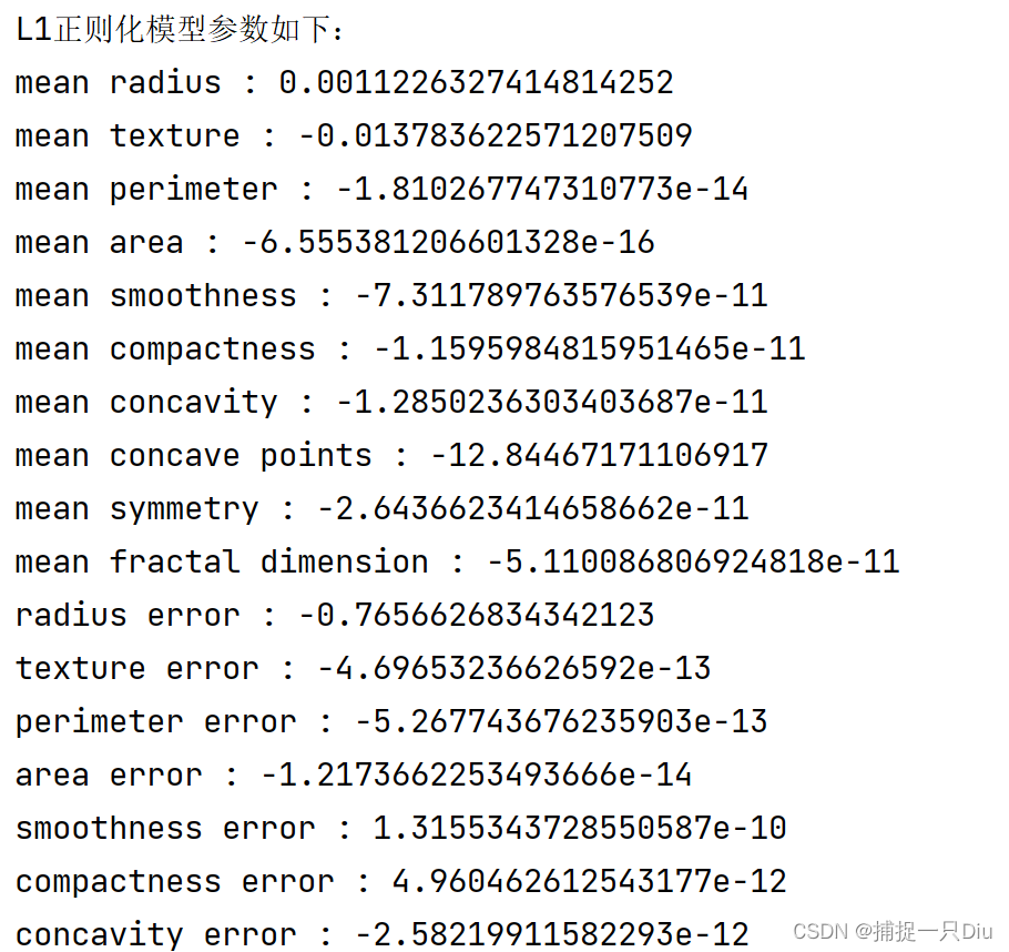
print("L1正则化模型参数如下:")
theta = lg_lr.get_params()
fn = bc_data.feature_names
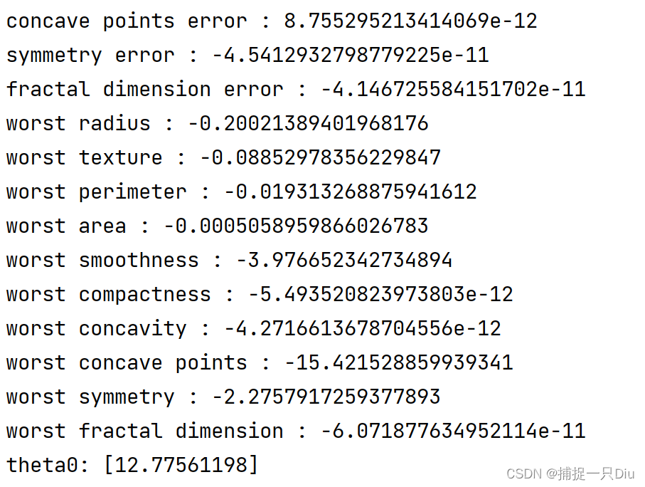
for i, w in enumerate(theta[0]):
print(fn[i], ":", w)
print("theta0:", theta[1])
print("=" * 70)
y_test_prob = lg_lr.predict_prob(X_test) # 预测概率
y_test_labels = lg_lr.predict(X_test)
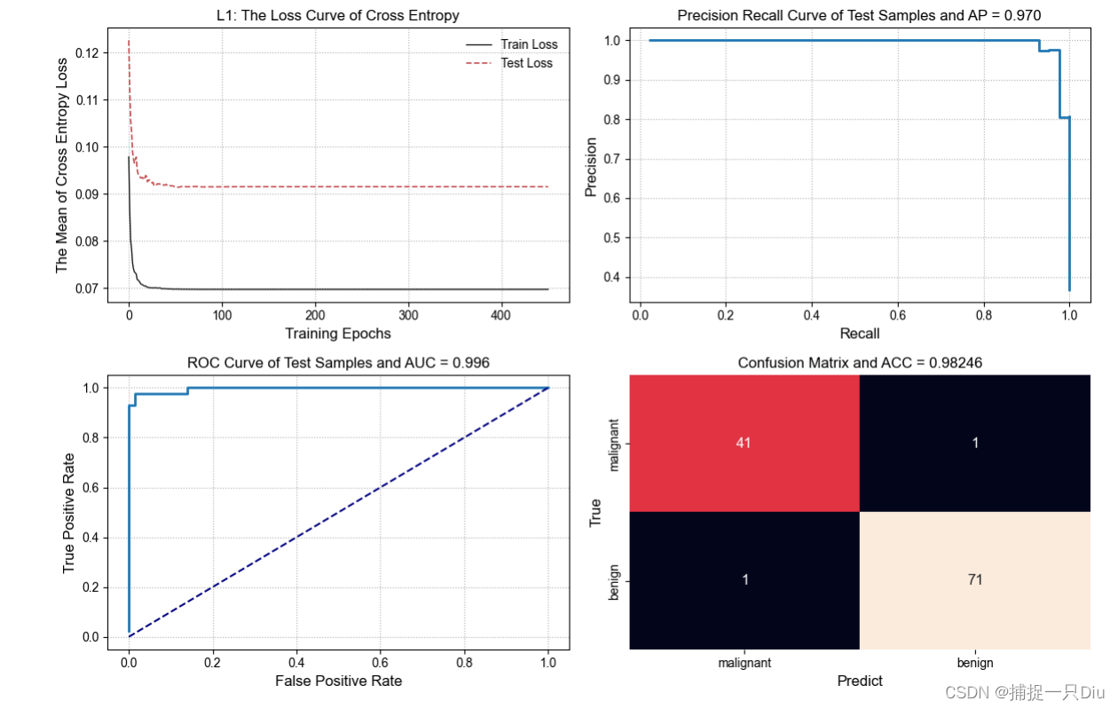
plt.figure(figsize=(12, 8))
plt.subplot(221)
lg_lr.plt_loss_curve(lab="L1", is_show=False)
pm = ModelPerformanceMetrics(y_test, y_test_prob)
print(pm.cal_classification_report())
pr_values = pm.precision_recall_curve() # PR指标值
plt.subplot(222)
pm.plt_pr_curve(pr_values, is_show=False) # PR曲线
roc_values = pm.roc_metrics_curve() # ROC指标值
plt.subplot(223)
pm.plt_roc_curve(roc_values, is_show=False) # ROC曲线
plt.subplot(224)
cm = pm.cal_confusion_matrix()
pm.plt_confusion_matrix(cm, label_names=["malignant", "benign"], is_show=False)
plt.tight_layout()
plt.show()
输出结果:


 5209
5209


 被折叠的 条评论
为什么被折叠?
被折叠的 条评论
为什么被折叠?
 到【灌水乐园】发言


